Mouse_Genome_Analysis

Mouse Genome Analysis

Upload Necessary Packages

library(ggplot2)
library(dplyr)
library(tidyverse)
library(MatchIt)
library(tidyr)
library(DescTools)
library(car)
library(PMCMRplus)
library(data.table)
library(sp)

Upload Necessary Files

#Upload Files

Top_buffered_mouse = "C:/Users/Aden Le/Documents/Cenik Lab/Research Project/Mousegenome/R-studio/Top_buffered_mouse.csv"
Top_buffered_mouse_data <- read.csv(Top_buffered_mouse)

Top2_buffered_mouse = "C:/Users/Aden Le/Documents/Cenik Lab/Research Project/Mousegenome/R-studio/Top2_buffered_mouse.csv"
Top2_buffered_mouse_data <- read.csv(Top2_buffered_mouse)

Mouse_stats_path = "C:/Users/Aden Le/Documents/Cenik Lab/Research Project/Mousegenome/R-studio/Mouse_statsR.csv"
Mouse_stats <- read.csv(Mouse_stats_path)

Tidy the Dataset

#Tidying the Data set

# Capitalize the 'transcript' column
Mouse_stats <- Mouse_stats %>%
  mutate(transcript = toupper(transcript))

# Change 0's to 1's in specific columns (e.g., Column1, Column2, Column3) so log(1) = 0
Mouse_stats <- Mouse_stats %>%
  mutate(UTR3_GC = ifelse(UTR3_GC == 0, 1, UTR3_GC),
         UTR3_len = ifelse(UTR3_len == 0, 1, UTR3_len),
         UTR5_GC = ifelse(UTR5_GC == 0, 1, UTR5_GC),
         UTR5_len = ifelse(UTR5_len == 0, 1, UTR5_len),
         CDS_GC = ifelse(CDS_GC == 0, 1, CDS_GC),
         CDS_len = ifelse(CDS_len == 0, 1, CDS_len)
         )

Mouse_stats <- Mouse_stats %>%
  mutate(UTR3_GC = log10(UTR3_GC),
         UTR3_len = log10(UTR3_len),
         UTR5_GC = log10(UTR5_GC),
         UTR5_len = log10(UTR5_len),
         CDS_GC = log10(CDS_GC),
         CDS_len = log10(CDS_len)
         )

CDS GC Percentage with (UTR3 + UTR5 Percentage Matchit)


Mouse_stats_Match_Prep <- Mouse_stats |>
  mutate(Buffering = if_else(transcript %in% Top_buffered_mouse_data$transcript, "TB1",
                             if_else(transcript %in% Top2_buffered_mouse_data$transcript, "TB2", "TB3"))) |>
  select(Buffering, UTR3_GC_Perc, UTR5_GC_Perc, CDS_GC_Perc, transcript)


# Binary for Matchit TB1 & TB2 = 1 | TB3 = 0
Mouse_stats_Match_Prep <- as.data.table(Mouse_stats_Match_Prep)
Mouse_stats_Match_Prep[, treat := ifelse(Buffering %in% c("TB1", "TB2"), 1, 0)]

#remove NA
Mouse_stats_Match_Prep <- na.omit(Mouse_stats_Match_Prep)

# Matches based on UTR3_GC_Perc + UTR5_GC_Perc
m.out <- matchit(treat ~ UTR3_GC_Perc + UTR5_GC_Perc, Mouse_stats_Match_Prep, method = "nearest")
  #summary(m.out)

data_matched <- match.data(m.out)

data_matched_long <- pivot_longer(data_matched, cols = c(CDS_GC_Perc), names_to = "Variable", values_to = "Value") |>
  select(Value, Variable, Buffering, transcript)

Visualize

# Define the levels for comparison
data_matched_long$Buffering <- factor(data_matched_long$Buffering, levels = c("TB1","TB2","TB3"))


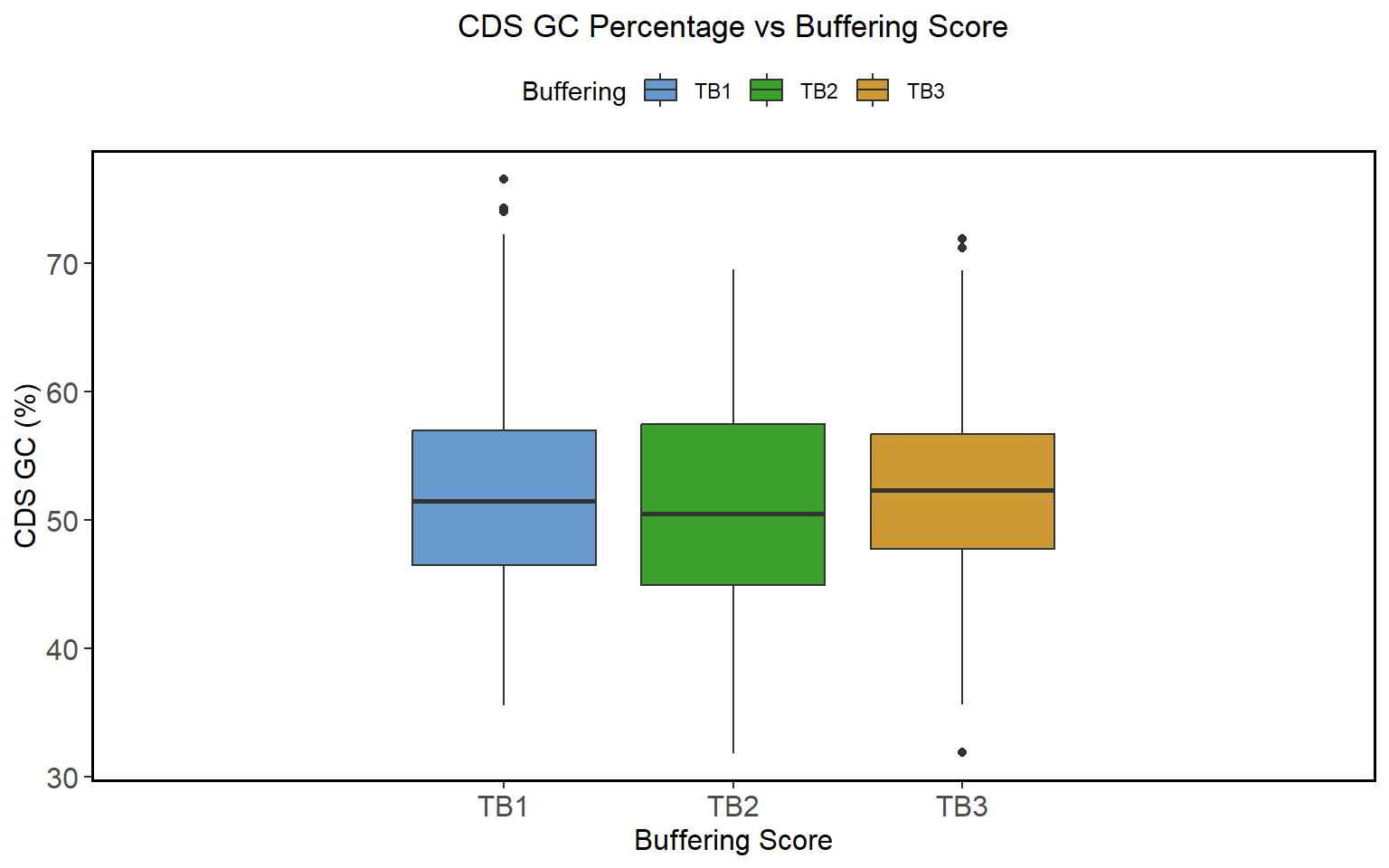
ggplot(data_matched_long, aes(x = Buffering, y = Value, fill = Buffering)) +
  geom_boxplot(width = 0.8, position = position_dodge(width = 0.9)) + # Adjust width and dodge width
  scale_fill_manual(values = c("#6699CC", "#3aa12b", "#CC9933")) +
  scale_x_discrete(expand = c(0.9, 0)) + # Reduce the expansion on the x-axis
  labs(title = "CDS GC Percentage vs Buffering Score", x = "Buffering Score", y = "CDS GC (%)") +
  
  theme(
      axis.text = element_text(size = 12),
      axis.title = element_text(size = 12),
      plot.title = element_text(hjust = 0.5),
      panel.background = element_rect(fill = "white"),
      panel.grid = element_blank(),
      panel.border = element_rect(color = "black", size = 1, fill = NA),
      panel.spacing = unit(0.5, "lines"),
      legend.position = "top"  # Position the legend at the top
    )

Significance Test

group1 <- filter(data_matched_long, Buffering == "TB1") |>
  select(Value)
group2 <- filter(data_matched_long, Buffering == "TB2") |>
  select(Value)
group3 <- filter(data_matched_long, Buffering == "TB3") |>
  select(Value)



group1_transform <- log(as.numeric(unlist(group1)))
group2_transform <- log(as.numeric(unlist(group2)))
group3_transform <- log(as.numeric(unlist(group3)))
#If the deviation is zero, to avoid infinite values after logarithmic conversion, make the deviation a super small number
#group3[group3 == 0] <- 1e-10  

# Combine the groups into a data frame for testing
data_combined <- data.frame(
  value = c(group1_transform, group2_transform, group3_transform),
  group = factor(rep(c("Group 1", "Group 2", "Group 3"), 
                     c(length(group1_transform), length(group2_transform), length(group3_transform))))
)

# Check normality for each group with a Shapiro test and visualize with a qqline plot
shapiro_test_group1 <- shapiro.test(group1_transform)
shapiro_test_group1

    Shapiro-Wilk normality test

data:  group1_transform
W = 0.99297, p-value = 0.2854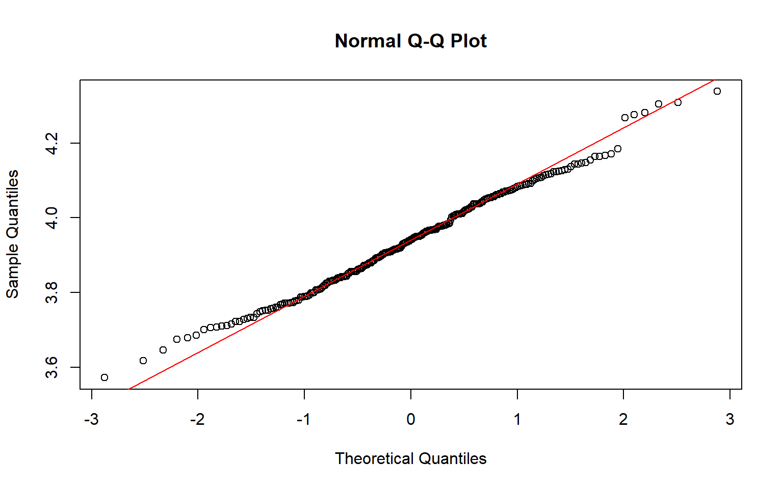


qqnorm(group1_transform)                  
qqline(group1_transform, col = "red")


shapiro_test_group2 <- shapiro.test(group2_transform)
shapiro_test_group2

    Shapiro-Wilk normality test

data:  group2_transform
W = 0.98624, p-value = 0.01666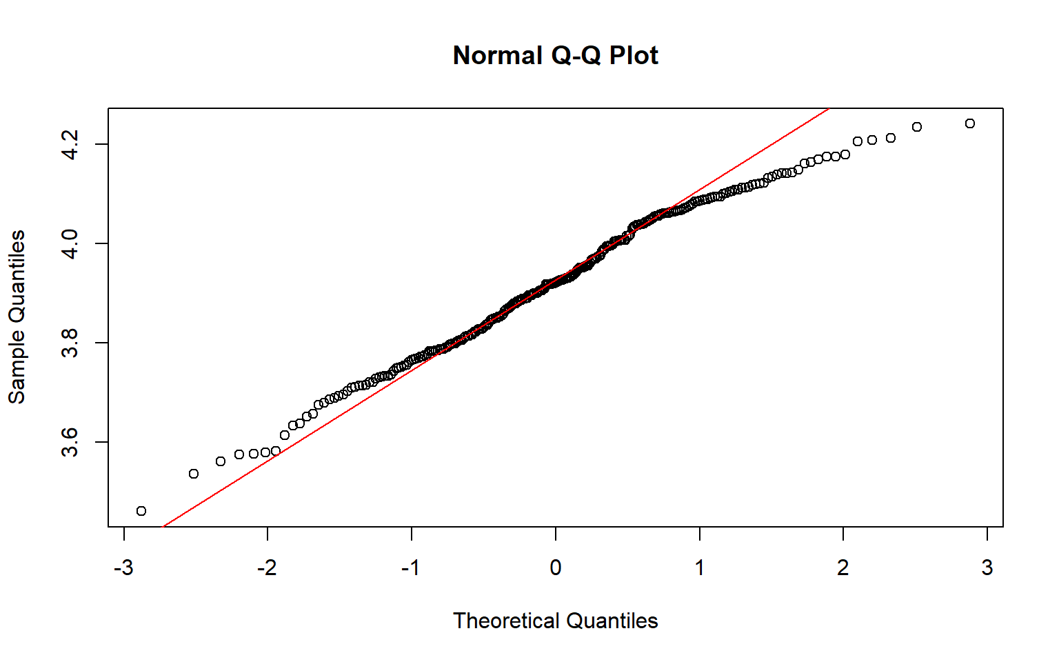


qqnorm(group2_transform)          
qqline(group2_transform, col = "red")


shapiro_test_group3 <- shapiro.test(group3_transform)
shapiro_test_group3

    Shapiro-Wilk normality test

data:  group3_transform
W = 0.99016, p-value = 0.001999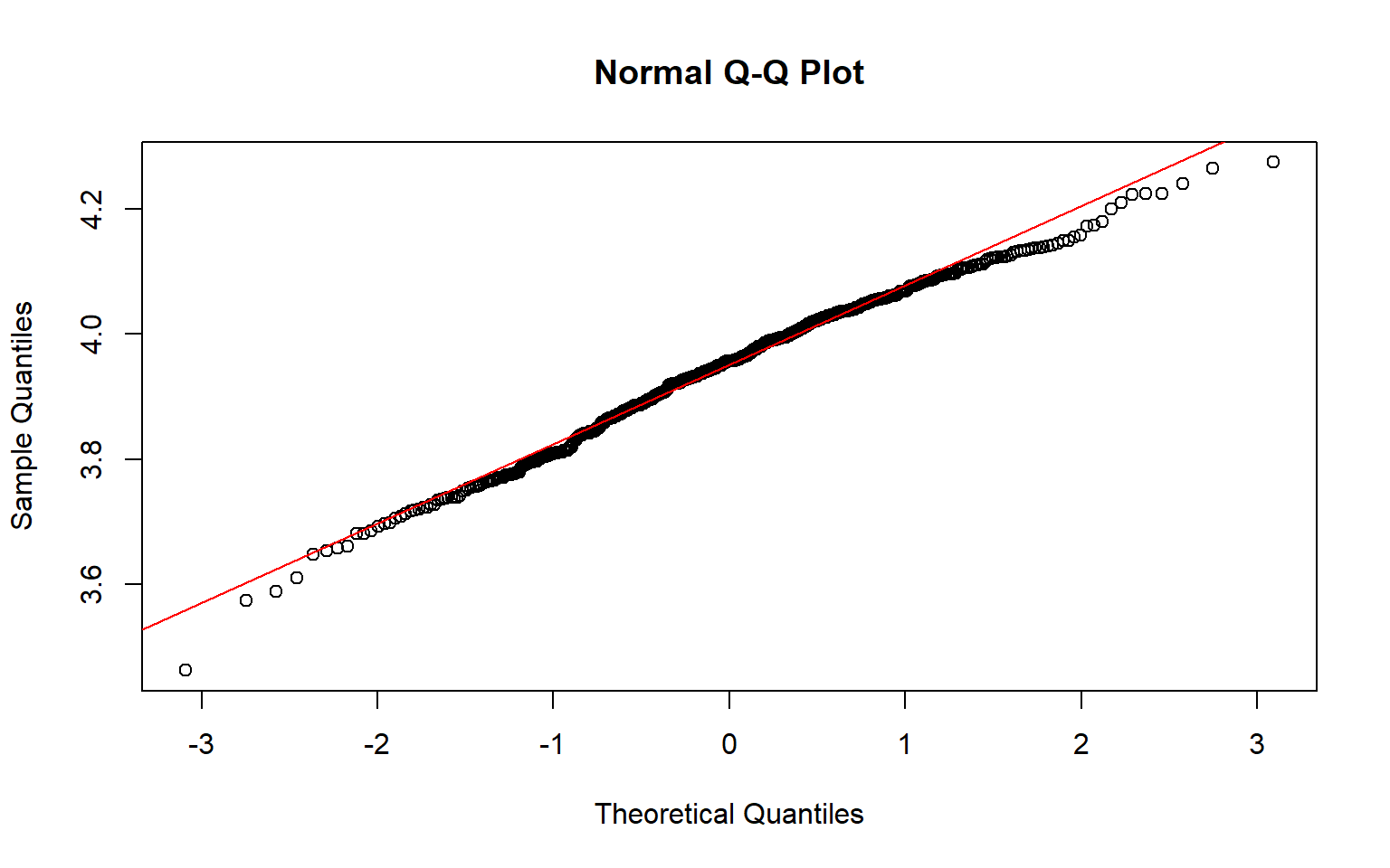


qqnorm(group3_transform)                  
qqline(group3_transform, col = "red")


# Levene test shoud be greater than 0.05 to indicate normal distribution
levene_test_result <- leveneTest(value ~ group, data = data_combined)
levene_test_result
Levene's Test for Homogeneity of Variance (center = median)
       Df F value    Pr(>F)    
group   2   8.655 0.0001877 ***
      997                      
---
Signif. codes:  0 '***' 0.001 '**' 0.01 '*' 0.05 '.' 0.1 ' ' 1


# Welch Anova test, doesn't assume equal variance or equal sample sizes
welch_anova_result <- oneway.test(value ~ group, data = data_combined)
welch_anova_result

    One-way analysis of means (not assuming equal variances)

data:  value and group
F = 2.9498, num df = 2.00, denom df = 499.86, p-value = 0.05326


# Games-Howell test, doesn't assume equal variance or equal sample sizes
games_howell_result <- gamesHowellTest(value ~ group, data = data_combined)
print(games_howell_result)
        Group 1 Group 2
Group 2 0.287   -      
Group 3 0.755   0.041

CDS Len with (UTR3 + UTR5 Len Matchit)


#Match-It

Mouse_stats_Match_Prep <- Mouse_stats |>
  mutate(Buffering = if_else(transcript %in% Top_buffered_mouse_data$transcript, "TB1",
                             if_else(transcript %in% Top2_buffered_mouse_data$transcript, "TB2", "TB3"))) |>
  select(Buffering, UTR5_len, UTR3_len, CDS_len, transcript)


# Binary for Matchit TB1 & TB2 = 1 | TB3 = 0
Mouse_stats_Match_Prep <- as.data.table(Mouse_stats_Match_Prep)
Mouse_stats_Match_Prep[, treat := ifelse(Buffering %in% c("TB1", "TB2"), 1, 0)]

#remove NA
Mouse_stats_Match_Prep <- na.omit(Mouse_stats_Match_Prep)

# Matches based on UTR3_GC_Perc + UTR5_GC_Perc
m.out <- matchit(treat ~ UTR3_len + UTR5_len, Mouse_stats_Match_Prep, method = "nearest")
#summary(m.out)

data_matched <- match.data(m.out)

data_matched_long <- pivot_longer(data_matched, cols = c(CDS_len), names_to = "Variable", values_to = "Value") |>
  select(Value, Variable, Buffering, transcript)

Visualize

# Define the levels for comparison
data_matched_long$Buffering <- factor(data_matched_long$Buffering, levels = c("TB1","TB2","TB3"))


ggplot(data_matched_long, aes(x = Buffering, y = Value, fill = Buffering)) +
  geom_boxplot(width = 0.8, position = position_dodge(width = 0.9)) + # Adjust width and dodge width
  scale_fill_manual(values = c("#6699CC", "#3aa12b", "#CC9933")) +
  scale_x_discrete(expand = c(0.9, 0)) + # Reduce the expansion on the x-axis
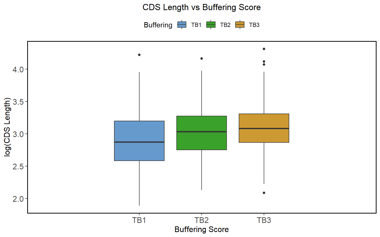
  labs(title = "CDS Length vs Buffering Score", x = "Buffering Score", y = "log(CDS Length)") +
  
  theme(
    axis.text = element_text(size = 12),
    axis.title = element_text(size = 12),
    plot.title = element_text(hjust = 0.5),
    panel.background = element_rect(fill = "white"),
    panel.grid = element_blank(),
    panel.border = element_rect(color = "black", size = 1, fill = NA),
    panel.spacing = unit(0.5, "lines"),
    legend.position = "top"  # Position the legend at the top
  )

Significance Test

group1 <- filter(data_matched_long, Buffering == "TB1") |>
  select(Value)
group2 <- filter(data_matched_long, Buffering == "TB2") |>
  select(Value)
group3 <- filter(data_matched_long, Buffering == "TB3") |>
  select(Value)

group1_transform <- log(as.numeric(unlist(group1)))
group2_transform <- log(as.numeric(unlist(group2)))
group3_transform <- log(as.numeric(unlist(group3)))
#If the deviation is zero, to avoid infinite values after logarithmic conversion, make the deviation a super small number
#group3[group3 == 0] <- 1e-10  

# Combine the groups into a data frame for testing
data_combined <- data.frame(
  value = c(group1_transform, group2_transform, group3_transform),
  group = factor(rep(c("Group 1", "Group 2", "Group 3"), 
                     c(length(group1_transform), length(group2_transform), length(group3_transform))))
)

# Check normality for each group with a Shapiro test and visualize with a qqline plot
shapiro_test_group1 <- shapiro.test(group1_transform)
shapiro_test_group1

    Shapiro-Wilk normality test

data:  group1_transform
W = 0.99264, p-value = 0.2508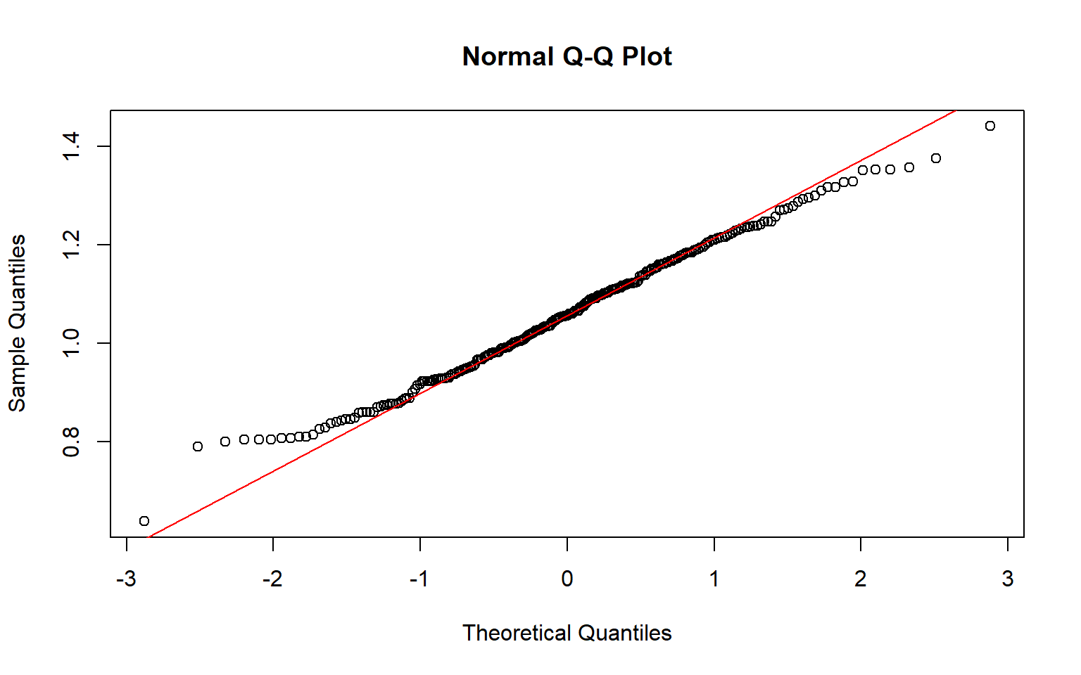


qqnorm(group1_transform)                  
qqline(group1_transform, col = "red")


shapiro_test_group2 <- shapiro.test(group2_transform)
shapiro_test_group2

    Shapiro-Wilk normality test

data:  group2_transform
W = 0.99304, p-value = 0.2943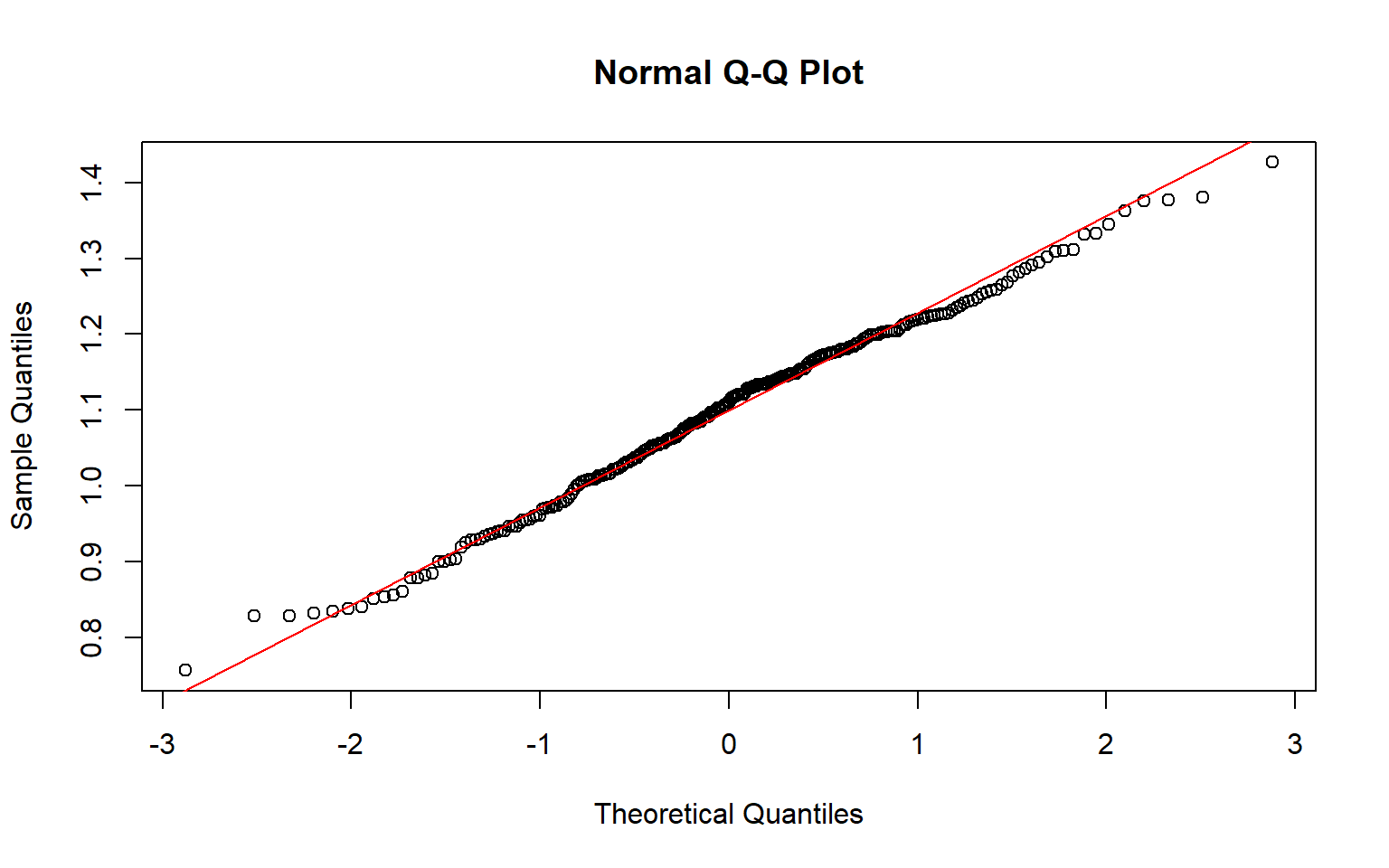


qqnorm(group2_transform)          
qqline(group2_transform, col = "red")


shapiro_test_group3 <- shapiro.test(group3_transform)
shapiro_test_group3

    Shapiro-Wilk normality test

data:  group3_transform
W = 0.99692, p-value = 0.4663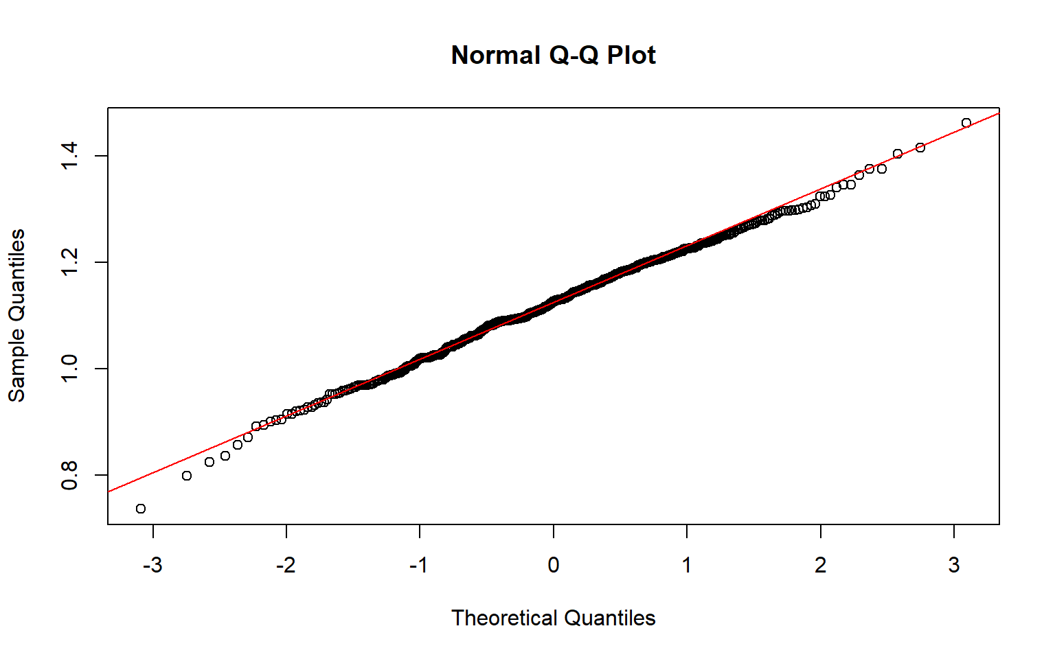


qqnorm(group3_transform)                  
qqline(group3_transform, col = "red")


# Levene test shoud be greater than 0.05 to indicate normal distribution
levene_test_result <- leveneTest(value ~ group, data = data_combined)
levene_test_result
Levene's Test for Homogeneity of Variance (center = median)
       Df F value    Pr(>F)    
group   2  18.135 1.837e-08 ***
      997                      
---
Signif. codes:  0 '***' 0.001 '**' 0.01 '*' 0.05 '.' 0.1 ' ' 1


# Welch Anova test, doesn't assume equal variance or equal sample sizes
welch_anova_result <- oneway.test(value ~ group, data = data_combined)
welch_anova_result

    One-way analysis of means (not assuming equal variances)

data:  value and group
F = 20.508, num df = 2.00, denom df = 482.95, p-value = 2.828e-09


# Games-Howell test, doesn't assume equal variance or equal sample sizes
games_howell_result <- gamesHowellTest(value ~ group, data = data_combined)
print(games_howell_result)
        Group 1 Group 2
Group 2 0.0023  -      
Group 3 2.2e-09 0.0269

UTR Len with (CDS Len Matchit)


#Match-It

Mouse_stats_Match_Prep <- Mouse_stats |>
  mutate(Buffering = if_else(transcript %in% Top_buffered_mouse_data$transcript, "TB1",
                             if_else(transcript %in% Top2_buffered_mouse_data$transcript, "TB2", "TB3"))) |>
  select(Buffering, UTR5_len, UTR3_len, CDS_len, transcript)


# Binary for Matchit TB1 & TB2 = 1 | TB3 = 0
Mouse_stats_Match_Prep <- as.data.table(Mouse_stats_Match_Prep)
Mouse_stats_Match_Prep[, treat := ifelse(Buffering %in% c("TB1", "TB2"), 1, 0)]

#remove NA
Mouse_stats_Match_Prep <- na.omit(Mouse_stats_Match_Prep)

# Matches based on UTR3_GC_Perc + UTR5_GC_Perc
m.out <- matchit(treat ~ CDS_len, Mouse_stats_Match_Prep, method = "nearest")
#summary(m.out)

data_matched <- match.data(m.out)

data_matched_long <- pivot_longer(data_matched, cols = c(UTR5_len, UTR3_len), names_to = "Variable", values_to = "Value") |>
  select(Value, Variable, Buffering, transcript)

Visualize

#Match-It

# Define the levels for comparison
data_matched_long$Buffering <- factor(data_matched_long$Buffering, levels = c("TB1","TB2","TB3"))

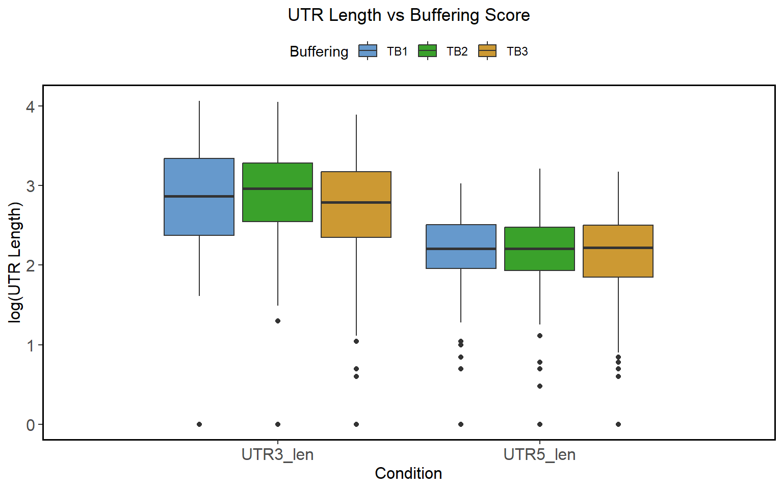
ggplot(data_matched_long, aes(x = Variable, y = Value, fill = Buffering)) +
  geom_boxplot(width = 0.8, position = position_dodge(width = 0.9)) + # Adjust width and dodge width
  scale_fill_manual(values = c("#6699CC", "#3aa12b", "#CC9933")) +
  scale_x_discrete(expand = c(0.9, 0)) + # Reduce the expansion on the x-axis
  labs(title = "UTR Length vs Buffering Score", x = "Condition", y = "log(UTR Length)") +
  
  theme(
    axis.text = element_text(size = 12),
    axis.title = element_text(size = 12),
    plot.title = element_text(hjust = 0.5),
    panel.background = element_rect(fill = "white"),
    panel.grid = element_blank(),
    panel.border = element_rect(color = "black", size = 1, fill = NA),
    panel.spacing = unit(0.5, "lines"),
    legend.position = "top"  # Position the legend at the top
  )

Significance Test UTR3

data_matched_long_UTR3 <- data_matched_long |>
  filter(Variable == "UTR3_len") |>
  filter(Value != 0)

group1 <- filter(data_matched_long_UTR3, Buffering == "TB1") |>
  select(Value)

group2 <- filter(data_matched_long_UTR3, Buffering == "TB2") |>
  select(Value)
group3 <- filter(data_matched_long_UTR3, Buffering == "TB3") |>
  select(Value)

group1_transform <- log(as.numeric(unlist(group1)))
group2_transform <- log(as.numeric(unlist(group2)))
group3_transform <- log(as.numeric(unlist(group3)))
#If the deviation is zero, to avoid infinite values after logarithmic conversion, make the deviation a super small number

# Combine the groups into a data frame for testing
data_combined <- data.frame(
  value = c(group1_transform, group2_transform, group3_transform),
  group = factor(rep(c("Group 1", "Group 2", "Group 3"), 
                     c(length(group1_transform), length(group2_transform), length(group3_transform))))
)

# Check normality for each group with a Shapiro test and visualize with a qqline plot
shapiro_test_group1 <- shapiro.test(group1_transform)
shapiro_test_group1

    Shapiro-Wilk normality test

data:  group1_transform
W = 0.96589, p-value = 1.211e-05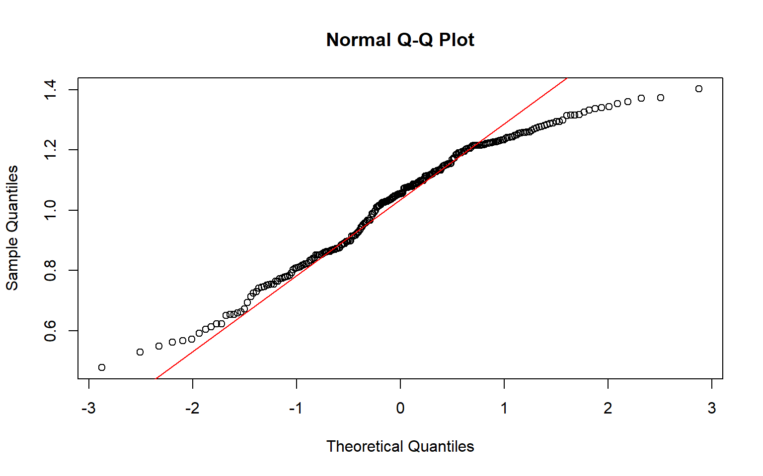


qqnorm(group1_transform)                  
qqline(group1_transform, col = "red")


shapiro_test_group2 <- shapiro.test(group2_transform)
shapiro_test_group2

    Shapiro-Wilk normality test

data:  group2_transform
W = 0.93537, p-value = 6.038e-09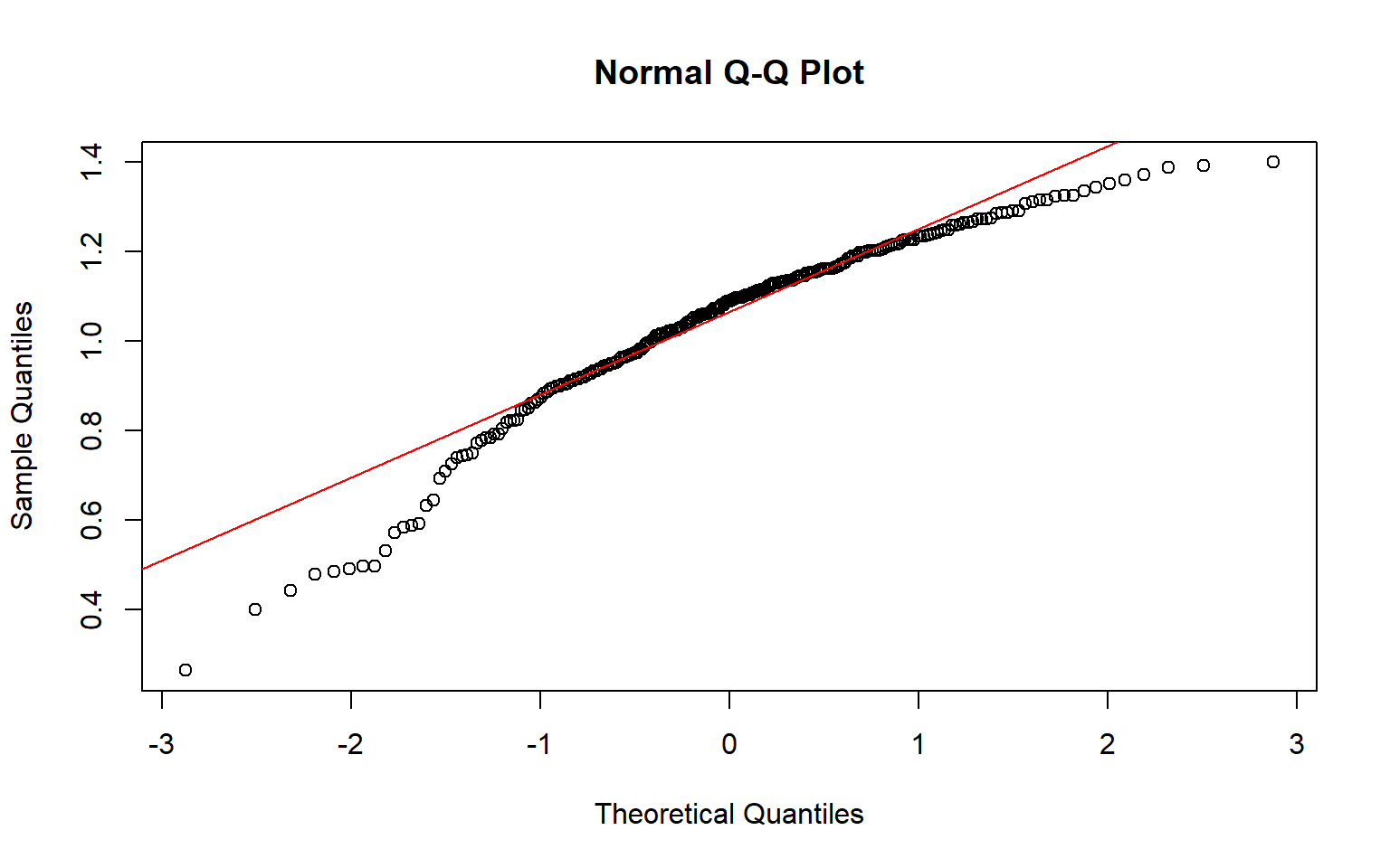


qqnorm(group2_transform)          
qqline(group2_transform, col = "red")


shapiro_test_group3 <- shapiro.test(group3_transform)
shapiro_test_group3

    Shapiro-Wilk normality test

data:  group3_transform
W = 0.89529, p-value < 2.2e-16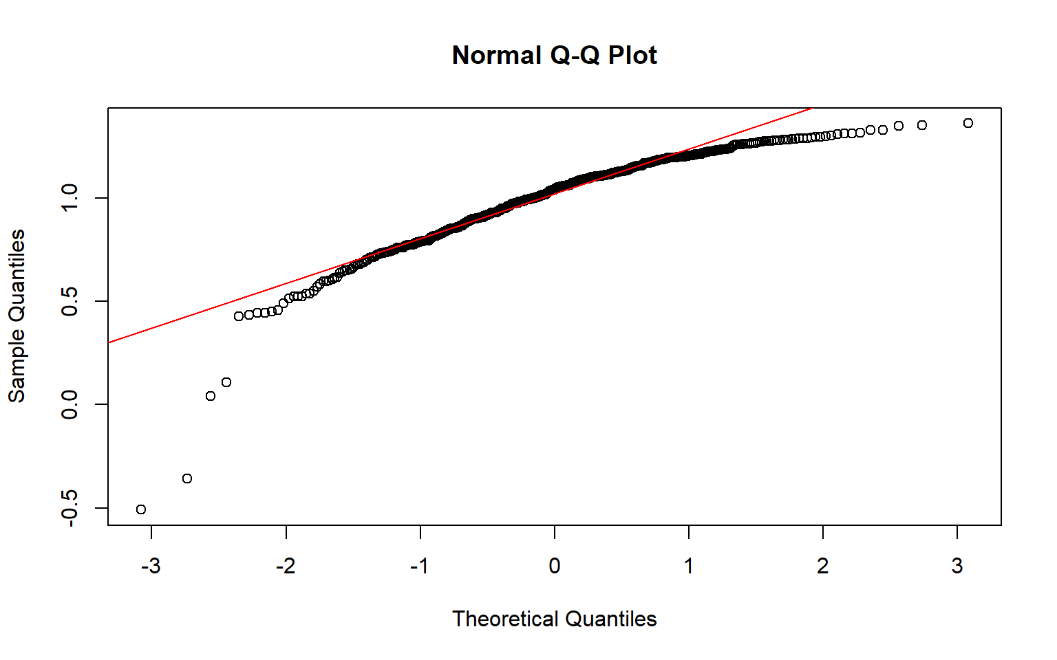


qqnorm(group3_transform)                  
qqline(group3_transform, col = "red")


# Levene test shoud be greater than 0.05 to indicate normal distribution
levene_test_result <- leveneTest(value ~ group, data = data_combined)
levene_test_result
Levene's Test for Homogeneity of Variance (center = median)
       Df F value Pr(>F)
group   2  1.1583 0.3145
      974


# Welch Anova test, doesn't assume equal variance or equal sample sizes
welch_anova_result <- oneway.test(value ~ group, data = data_combined)
welch_anova_result

    One-way analysis of means (not assuming equal variances)

data:  value and group
F = 4.2133, num df = 2.00, denom df = 546.75, p-value = 0.01528


# Games-Howell test, doesn't assume equal variance or equal sample sizes
games_howell_result <- gamesHowellTest(value ~ group, data = data_combined)
print(games_howell_result)
        Group 1 Group 2
Group 2 0.535   -      
Group 3 0.226   0.013

Significance UTR5

data_matched_long_UTR5 <- data_matched_long |>
  filter(Variable == "UTR5_len") |>
  filter(Value != 0)

group1 <- filter(data_matched_long_UTR5, Buffering == "TB1") |>
  select(Value)

group2 <- filter(data_matched_long_UTR5, Buffering == "TB2") |>
  select(Value)
group3 <- filter(data_matched_long_UTR5, Buffering == "TB3") |>
  select(Value)

group1_transform <- log(as.numeric(unlist(group1)))
group2_transform <- log(as.numeric(unlist(group2)))
group3_transform <- log(as.numeric(unlist(group3)))
#If the deviation is zero, to avoid infinite values after logarithmic conversion, make the deviation a super small number

# Combine the groups into a data frame for testing
data_combined <- data.frame(
  value = c(group1_transform, group2_transform, group3_transform),
  group = factor(rep(c("Group 1", "Group 2", "Group 3"), 
                     c(length(group1_transform), length(group2_transform), length(group3_transform))))
)

# Check normality for each group with a Shapiro test and visualize with a qqline plot
shapiro_test_group1 <- shapiro.test(group1_transform)
shapiro_test_group1

    Shapiro-Wilk normality test

data:  group1_transform
W = 0.8767, p-value = 2.792e-13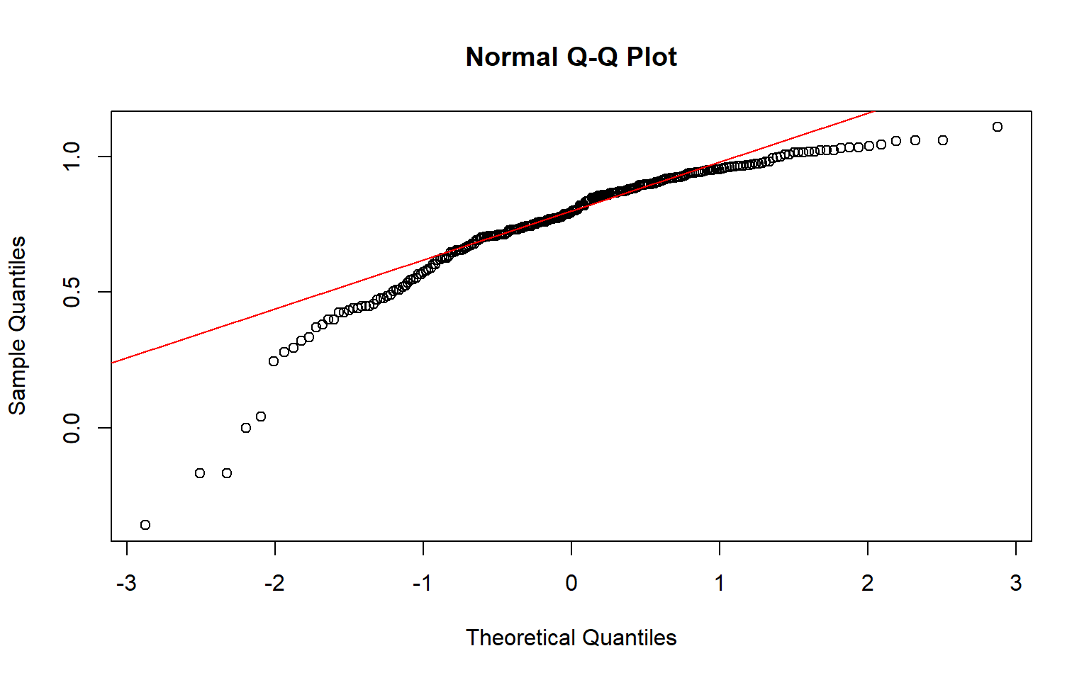


qqnorm(group1_transform)                  
qqline(group1_transform, col = "red")


shapiro_test_group2 <- shapiro.test(group2_transform)
shapiro_test_group2

    Shapiro-Wilk normality test

data:  group2_transform
W = 0.8527, p-value = 1.667e-14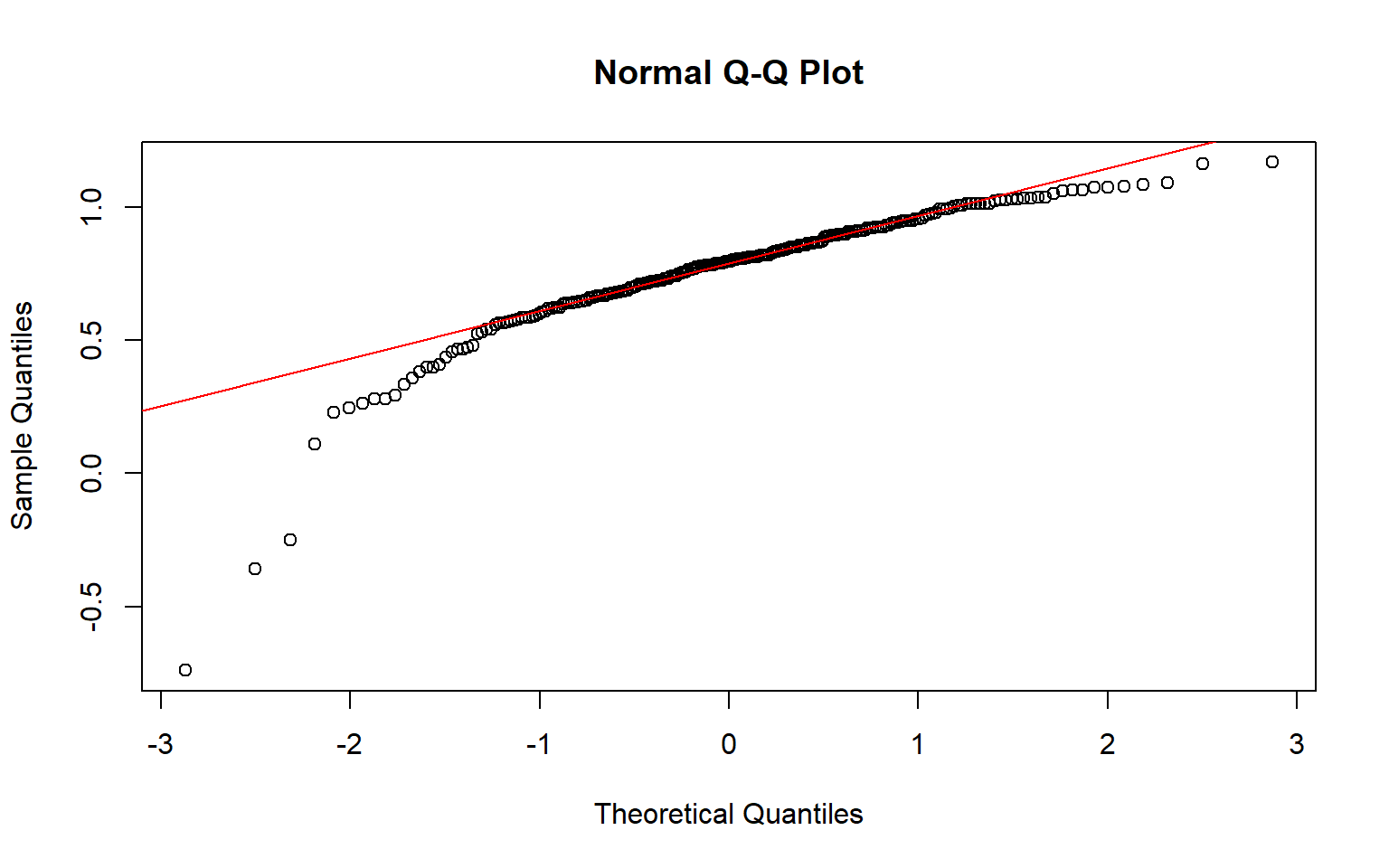


qqnorm(group2_transform)          
qqline(group2_transform, col = "red")


shapiro_test_group3 <- shapiro.test(group3_transform)
shapiro_test_group3

    Shapiro-Wilk normality test

data:  group3_transform
W = 0.88791, p-value < 2.2e-16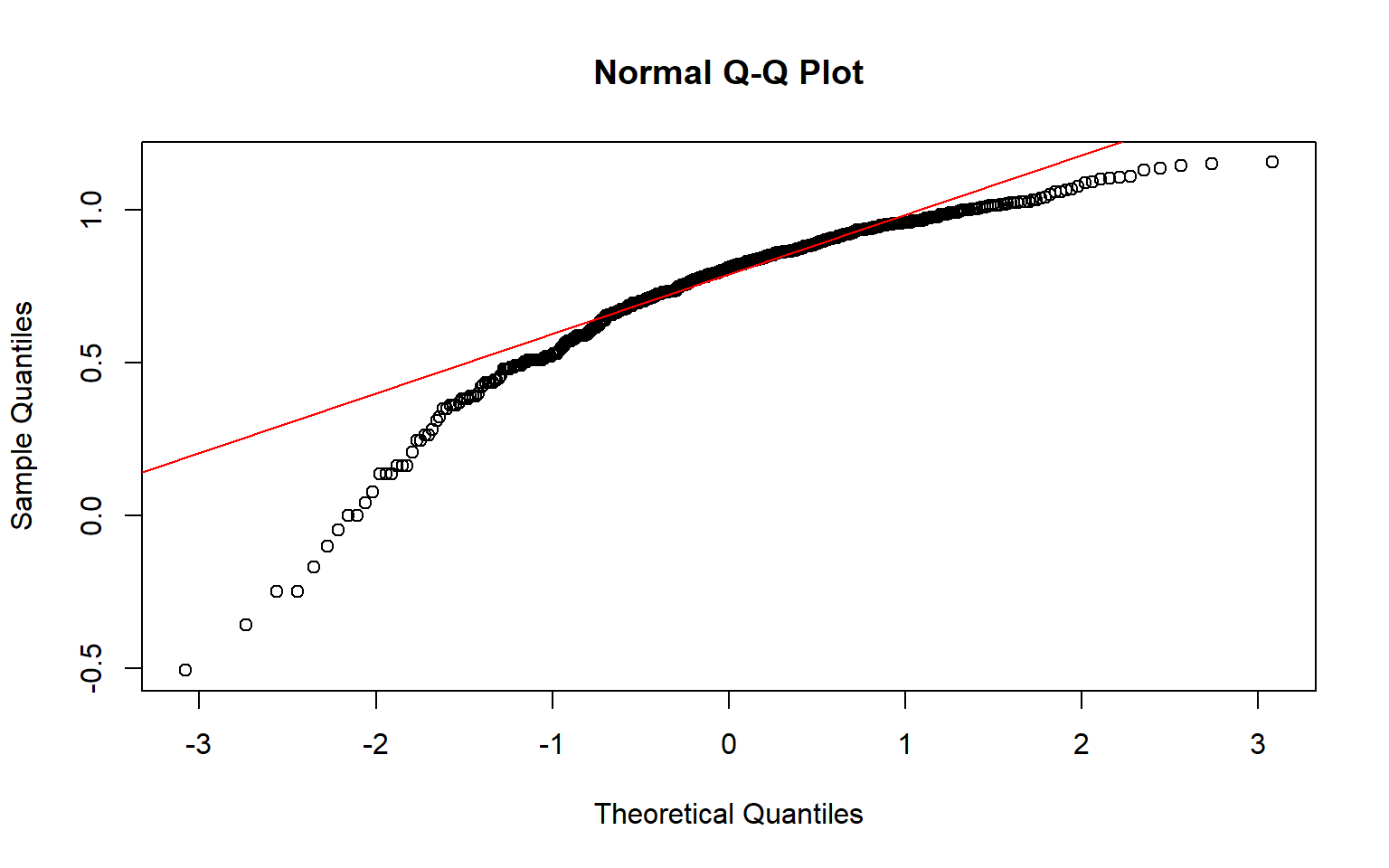


qqnorm(group3_transform)                  
qqline(group3_transform, col = "red")


# Levene test shoud be greater than 0.05 to indicate normal distribution
levene_test_result <- leveneTest(value ~ group, data = data_combined)
levene_test_result
Levene's Test for Homogeneity of Variance (center = median)
       Df F value Pr(>F)
group   2  0.9236 0.3974
      971


# Welch Anova test, doesn't assume equal variance or equal sample sizes
welch_anova_result <- oneway.test(value ~ group, data = data_combined)
welch_anova_result

    One-way analysis of means (not assuming equal variances)

data:  value and group
F = 0.24523, num df = 2.00, denom df = 537.59, p-value = 0.7826


# Games-Howell test, doesn't assume equal variance or equal sample sizes
games_howell_result <- gamesHowellTest(value ~ group, data = data_combined)
print(games_howell_result)
        Group 1 Group 2
Group 2 1.00    -      
Group 3 0.81    0.85

UTR3&5 GC Percentage with (CDS GC Percentage Matchit)

#Match-It

Mouse_stats_Match_Prep <- Mouse_stats |>
  mutate(Buffering = if_else(transcript %in% Top_buffered_mouse_data$transcript, "TB1",
                             if_else(transcript %in% Top2_buffered_mouse_data$transcript, "TB2", "TB3"))) |>
  select(Buffering, UTR3_GC_Perc, UTR5_GC_Perc, CDS_GC_Perc, transcript)


# Binary for Matchit TB1 & TB2 = 1 | TB3 = 0
Mouse_stats_Match_Prep <- as.data.table(Mouse_stats_Match_Prep)
Mouse_stats_Match_Prep[, treat := ifelse(Buffering %in% c("TB1", "TB2"), 1, 0)]

#remove NA
Mouse_stats_Match_Prep <- na.omit(Mouse_stats_Match_Prep)

# Matches based on UTR3_GC_Perc + UTR5_GC_Perc
m.out <- matchit(treat ~ CDS_GC_Perc, Mouse_stats_Match_Prep, method = "nearest")
#summary(m.out)

data_matched <- match.data(m.out)

data_matched_long <- pivot_longer(data_matched, cols = c(UTR3_GC_Perc, UTR5_GC_Perc), names_to = "Variable", values_to = "Value") |>
  select(Value, Variable, Buffering, transcript)

Visualize


# Define the levels for comparison
data_matched_long$Buffering <- factor(data_matched_long$Buffering, levels = c("TB1","TB2","TB3"))

ggplot(data_matched_long, aes(x = Variable, y = Value, fill = Buffering)) +
  geom_boxplot(width = 0.8, position = position_dodge(width = 0.9)) + # Adjust width and dodge width
  scale_fill_manual(values = c("#6699CC", "#3aa12b", "#CC9933")) +
  scale_x_discrete(expand = c(0.9, 0)) + # Reduce the expansion on the x-axis
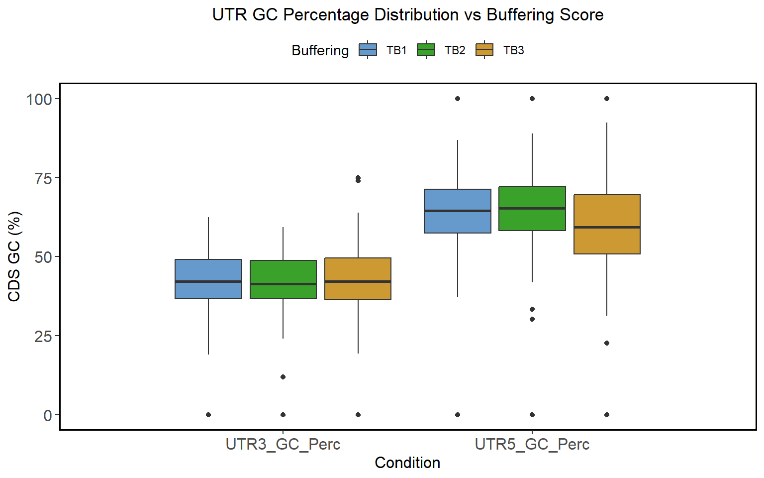
  labs(title = "UTR GC Percentage Distribution vs Buffering Score", x = "Condition", y = "CDS GC (%)") +
  
  theme(
    axis.text = element_text(size = 12),
    axis.title = element_text(size = 12),
    plot.title = element_text(hjust = 0.5),
    panel.background = element_rect(fill = "white"),
    panel.grid = element_blank(),
    panel.border = element_rect(color = "black", size = 1, fill = NA),
    panel.spacing = unit(0.5, "lines"),
    legend.position = "top"  # Position the legend at the top
  )

Significance Test UTR3

data_matched_long_UTR3 <- data_matched_long |>
  filter(Variable == "UTR3_GC_Perc") |>
  filter(Value != 0)

group1 <- filter(data_matched_long_UTR3, Buffering == "TB1") |>
  select(Value)

group2 <- filter(data_matched_long_UTR3, Buffering == "TB2") |>
  select(Value)
group3 <- filter(data_matched_long_UTR3, Buffering == "TB3") |>
  select(Value)

group1_transform <- log(as.numeric(unlist(group1)))
group2_transform <- log(as.numeric(unlist(group2)))
group3_transform <- log(as.numeric(unlist(group3)))
#If the deviation is zero, to avoid infinite values after logarithmic conversion, make the deviation a super small number

# Combine the groups into a data frame for testing
data_combined <- data.frame(
  value = c(group1_transform, group2_transform, group3_transform),
  group = factor(rep(c("Group 1", "Group 2", "Group 3"), 
                     c(length(group1_transform), length(group2_transform), length(group3_transform))))
)

# Check normality for each group with a Shapiro test and visualize with a qqline plot
shapiro_test_group1 <- shapiro.test(group1_transform)
shapiro_test_group1

    Shapiro-Wilk normality test

data:  group1_transform
W = 0.9821, p-value = 0.003247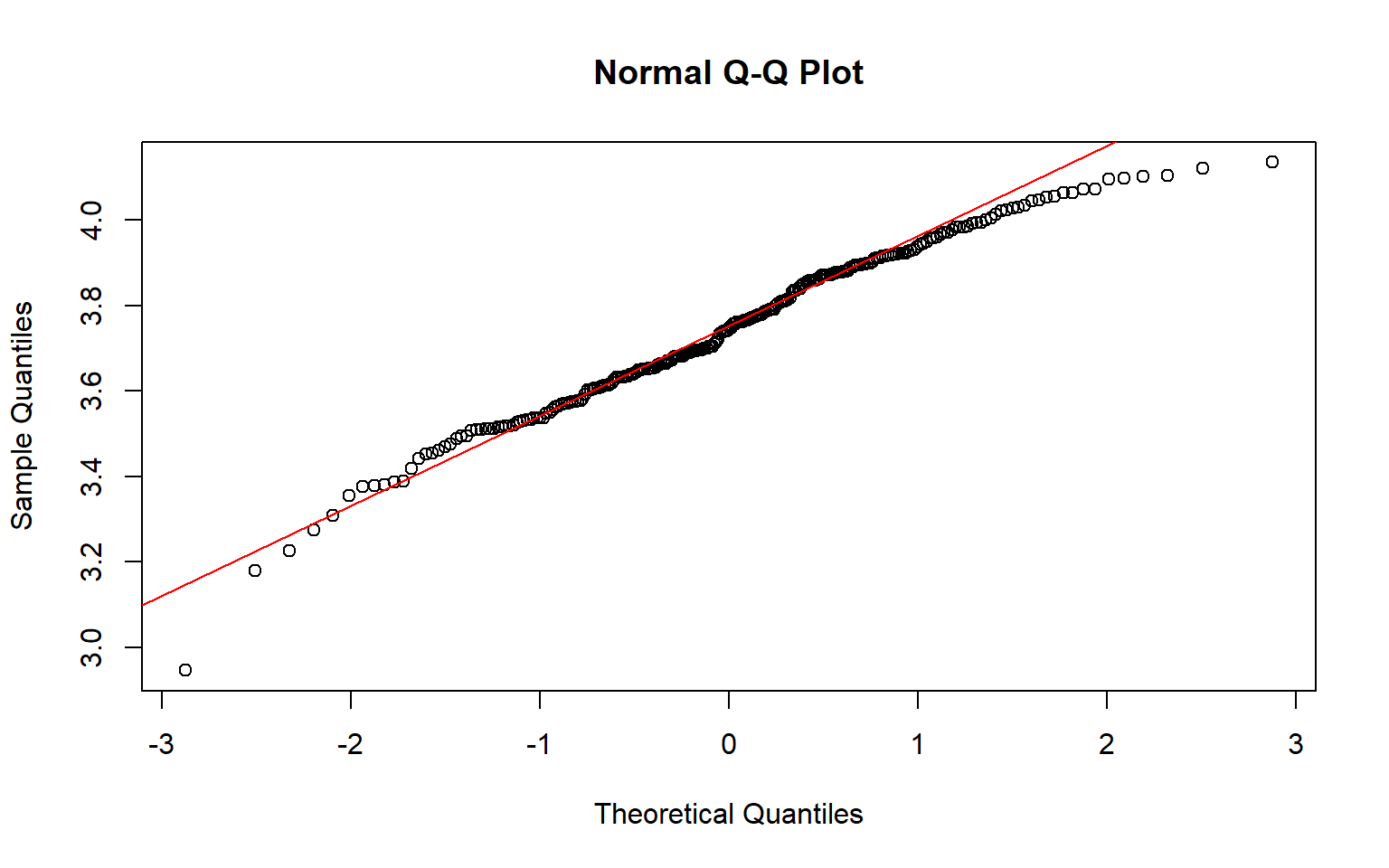


qqnorm(group1_transform)                  
qqline(group1_transform, col = "red")


shapiro_test_group2 <- shapiro.test(group2_transform)
shapiro_test_group2

    Shapiro-Wilk normality test

data:  group2_transform
W = 0.92984, p-value = 1.938e-09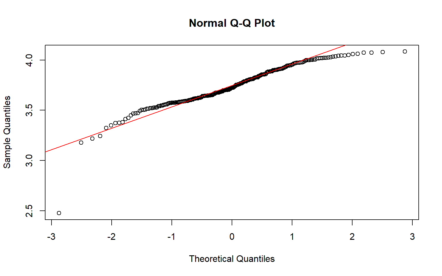


qqnorm(group2_transform)          
qqline(group2_transform, col = "red")


shapiro_test_group3 <- shapiro.test(group3_transform)
shapiro_test_group3

    Shapiro-Wilk normality test

data:  group3_transform
W = 0.97398, p-value = 1.472e-07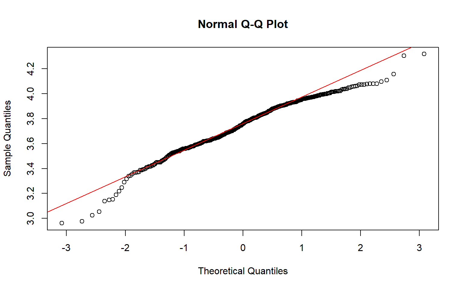


qqnorm(group3_transform)                  
qqline(group3_transform, col = "red")


# Levene test shoud be greater than 0.05 to indicate normal distribution
levene_test_result <- leveneTest(value ~ group, data = data_combined)
levene_test_result
Levene's Test for Homogeneity of Variance (center = median)
       Df F value Pr(>F)
group   2  0.4138 0.6612
      974


# Welch Anova test, doesn't assume equal variance or equal sample sizes
welch_anova_result <- oneway.test(value ~ group, data = data_combined)
welch_anova_result

    One-way analysis of means (not assuming equal variances)

data:  value and group
F = 0.064977, num df = 2.00, denom df = 534.24, p-value = 0.9371


# Games-Howell test, doesn't assume equal variance or equal sample sizes
games_howell_result <- gamesHowellTest(value ~ group, data = data_combined)
print(games_howell_result)
        Group 1 Group 2
Group 2 0.98    -      
Group 3 0.99    0.93

Significance Test UTR5

data_matched_long_UTR5 <- data_matched_long |>
  filter(Variable == "UTR5_GC_Perc") |>
  filter(Value != 0)

group1 <- filter(data_matched_long_UTR5, Buffering == "TB1") |>
  select(Value)

group2 <- filter(data_matched_long_UTR5, Buffering == "TB2") |>
  select(Value)
group3 <- filter(data_matched_long_UTR5, Buffering == "TB3") |>
  select(Value)

group1_transform <- log(as.numeric(unlist(group1)))
group2_transform <- log(as.numeric(unlist(group2)))
group3_transform <- log(as.numeric(unlist(group3)))
#If the deviation is zero, to avoid infinite values after logarithmic conversion, make the deviation a super small number

# Combine the groups into a data frame for testing
data_combined <- data.frame(
  value = c(group1_transform, group2_transform, group3_transform),
  group = factor(rep(c("Group 1", "Group 2", "Group 3"), 
                     c(length(group1_transform), length(group2_transform), length(group3_transform))))
)

# Check normality for each group with a Shapiro test and visualize with a qqline plot
shapiro_test_group1 <- shapiro.test(group1_transform)
shapiro_test_group1

    Shapiro-Wilk normality test

data:  group1_transform
W = 0.98743, p-value = 0.02868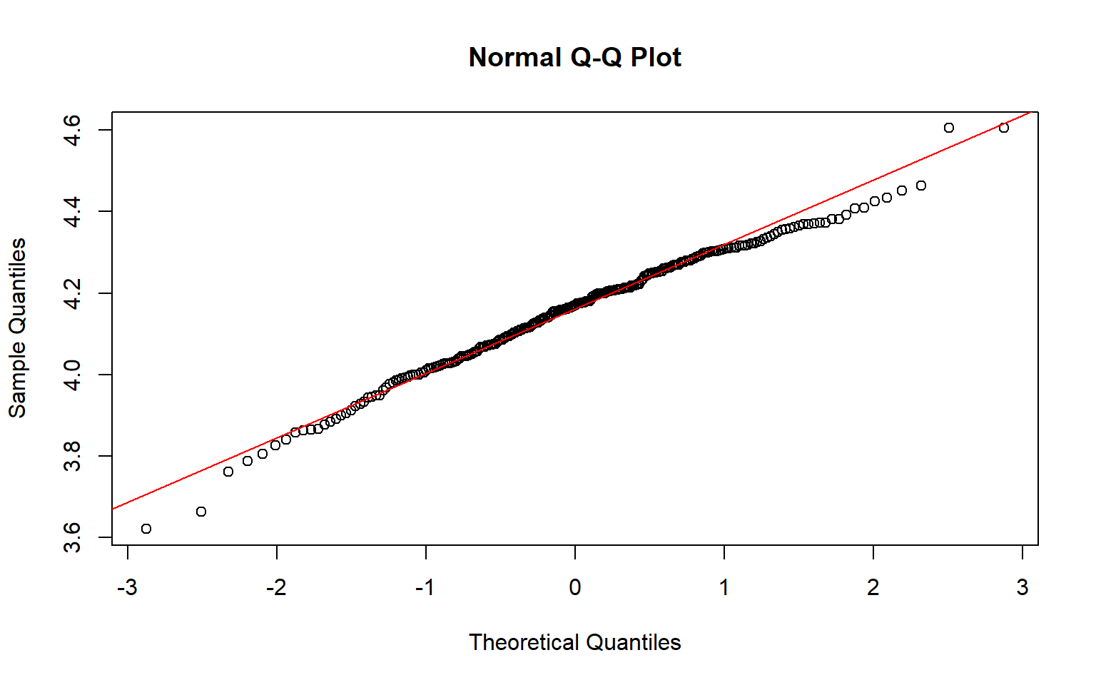


qqnorm(group1_transform)                  
qqline(group1_transform, col = "red")


shapiro_test_group2 <- shapiro.test(group2_transform)
shapiro_test_group2

    Shapiro-Wilk normality test

data:  group2_transform
W = 0.96438, p-value = 9.099e-06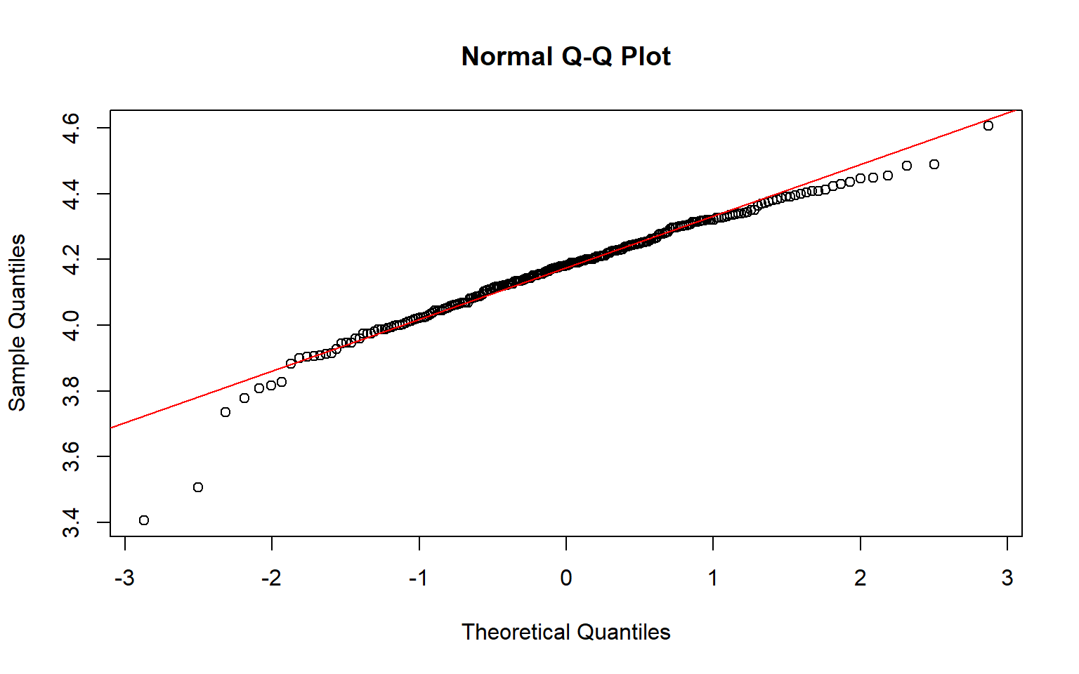


qqnorm(group2_transform)          
qqline(group2_transform, col = "red")


shapiro_test_group3 <- shapiro.test(group3_transform)
shapiro_test_group3

    Shapiro-Wilk normality test

data:  group3_transform
W = 0.97573, p-value = 4.014e-07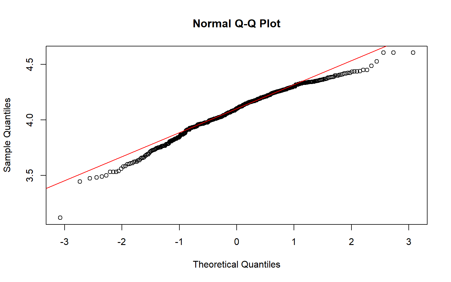


qqnorm(group3_transform)                  
qqline(group3_transform, col = "red")


# Levene test shoud be greater than 0.05 to indicate normal distribution
levene_test_result <- leveneTest(value ~ group, data = data_combined)
levene_test_result
Levene's Test for Homogeneity of Variance (center = median)
       Df F value    Pr(>F)    
group   2  28.133 1.332e-12 ***
      966                      
---
Signif. codes:  0 '***' 0.001 '**' 0.01 '*' 0.05 '.' 0.1 ' ' 1


# Welch Anova test, doesn't assume equal variance or equal sample sizes
welch_anova_result <- oneway.test(value ~ group, data = data_combined)
welch_anova_result

    One-way analysis of means (not assuming equal variances)

data:  value and group
F = 24.085, num df = 2.00, denom df = 588.08, p-value = 8.835e-11


# Games-Howell test, doesn't assume equal variance or equal sample sizes
games_howell_result <- gamesHowellTest(value ~ group, data = data_combined)
print(games_howell_result)
        Group 1 Group 2
Group 2 0.63    -      
Group 3 8.8e-08 6.3e-10

Brief Summary:

There is significant difference in the values for UTR5 GC content between the the buffered gene set and the non-buffered gene set.