RNA Flow ~ Human

Background Information:

MAP vs Mean:
- The mean is the average value of a probability distribution, representing the central tendency based purely on the data. In contrast, the MAP (Maximum A Posteriori) estimate is the most likely value of a parameter in Bayesian statistics, incorporating both the observed data and prior beliefs.
Extracted essential information for the analysis:
- Symbol: Gene Symbol
- PUND: Predicted to Undergo Nucleosome Degradation
- half_life_chr.Mean:
  - Mean (minutes) of how long RNA spends in the chromatin
  - half_life_nuc.Mean:
    - Mean (minutes) of how long RNA spends in the nucleoplasm
- half_life_cyto.Mean:
  - Mean (minutes) of how long RNA spends in the cytoplasm
- half_life_poly_entry.Mean:
  - Mean (minutes) of how long RNA remains available in the cytoplasm for potential translation before being degraded or otherwise processed.
- half_life_whole_cell.Mean
  - Mean (minutes) of the total time RNA spends in the whole cell.
- half_life_nucexp_from_nucres.MAP
  - MAP (minutes) of the time it takes to export Non-Pund genes out of the nucleus
- half_life_nucexp_from_nucdeg.MAP(PUND)
  - MAP (minutes of the time it takes to export PUND gene out of the nucleus

Visualizing the Data

Upload Necessary Packages

# Load necessary packages
library(ggplot2)
library(dplyr)
library(MatchIt)
library(tidyr)
library(DescTools)
library(car)
library(PMCMRplus)

Upload Necessary Files & Set Seed


# Set a seed for reproducibility
set.seed(56)

# Upload Buffered Gene Set
Buffering_Human_Data_Path <- "C:/Users/Aden Le/Documents/Cenik Lab/Research Project/RNA_flow/R_Stuff_Human/Human_Buffered_Genes.csv"
Buffering_Human_Data <- read.csv(Buffering_Human_Data_Path)

# Upload tidied Human Data
Human_Data_Path <- "C:/Users/Aden Le/Documents/Cenik Lab/Research Project/RNA_flow/R_Stuff_Human/Human_Data.csv"
Human_Data <- read.csv(Human_Data_Path)

#------------------------------------------------------------------
# Remove Excess Data
remove(Buffering_Human_Data_Path)
remove(Human_Data_Path)

Contains the average of the replicate means for all of the points of interest within the cell: Chromatin, Nucleoplasm, Cytoplasm, Polysome, and Whole Cell, Nuclear Export (PUND & Not PUND) & PUND Boolean

Rename and Reformat the Data


Human_Data$Match <- Human_Data$Symbol %in% Buffering_Human_Data$Symbo

#So I can left join it with the same column name
Buffering_Human_Data <- Buffering_Human_Data |>
  rename(
    "Symbol" = transcript
  )

#Combine the Human buffering set with the Human Gene Set | Formats the data for matching

Human_Data <- left_join(Human_Data, Buffering_Human_Data, by = "Symbol")

Renamed_Human_Data <- Human_Data |>
  rename(
    "Chromatin" = Chromatin.Average,
    "Nucleoplasm" = Nucleoplasm.Average,
    "Cytoplasm" = Cytoplasm.Average,
    "Untranslated Cytoplasm" = Polysome.Average
  )

Human_Data_matchit <- Renamed_Human_Data |>
  mutate(Buffering = case_when(
    
    is.na(Group) ~ "TB3",
    Group == "2" ~ "TB2",
    Group == "1" ~ "TB1",
    TRUE ~ NA_character_  # You can add a default case with TRUE if needed
    
  ))

Human_Data_matchit <- Human_Data_matchit %>%
  mutate(match_it_order = case_when(
    Buffering %in% c("TB1", "TB2") ~ 1,  # Assign 1 for Buffering values TB1 and TB2
    Buffering == "TB3" ~ 0,              # Assign 0 for Buffering value TB3
    TRUE ~ NA_real_                     # Handle other cases with NA_real_ for numeric NA
  ))

#------------------------------------------------------------------
# Remove Excess Data
remove(Buffering_Human_Data_Path)
remove(Human_Data_Path)

Formats the data in preparation for matching

Match the Data on Whole Cell Average


# Matches the data based on Whole Cell Average

m.out <- matchit(match_it_order ~ Whole.Cell.Average, data = Human_Data_matchit, method = "nearest")

# Get the matched data
data_matched_human <- match.data(m.out)


#Expands the data so it can be graphed
data_long <- pivot_longer(data_matched_human, 
                          cols = c("Chromatin", "Nucleoplasm", "Cytoplasm", "Untranslated Cytoplasm"), 
                          names_to = "Variable", 
                          values_to = "Value") |>
  select(Gene, Symbol, PUND, Variable, Value,Buffering)# Convert Value column to numeric



# Convert Value column to numeric
data_long$Value <- as.numeric(data_long$Value)

# Identify the rows with NA values in the Value column
na_rows <- which(is.na(data_long$Value))
# Remove rows where Value column has NA
data_long_clean <- data_long[!is.na(data_long$Value), ]

Plot the Data


data_long_clean$Buffering <- factor(data_long_clean$Buffering, levels = c("TB1","TB2","TB3"))

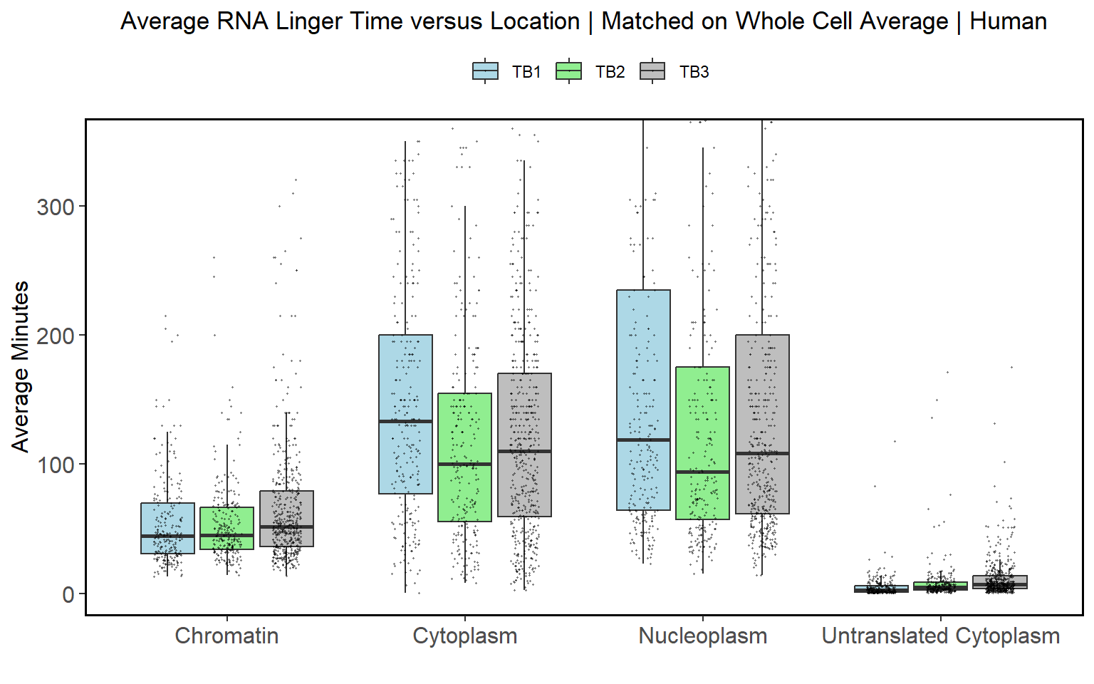
ggplot(data_long_clean, aes(Variable, Value, fill=factor(Buffering))) +
  geom_boxplot(outlier.shape = NA, outlier.colour = "black", outlier.size = 0, notch = FALSE) +
  geom_jitter(color = "black", size = 0.2, alpha = 0.4, position = position_jitterdodge(jitter.width = 0.3, dodge.width = 0.75)) +
  coord_cartesian(ylim = c(0, 350))+
  labs(
    title = "Average RNA Linger Time versus Location | Matched on Whole Cell Average | Human",
    x = "",  # x-axis label
    y = "Average Minutes",
    fill = ""  # Legend title
  ) +
  scale_fill_manual(
    values = c("lightblue", "lightgreen", "grey"),  # Example colors
    labels = c("TB1", "TB2", "TB3")  # Example labels
  ) +
  theme(
    axis.text = element_text(size = 12),
    axis.title = element_text(size = 12),
    plot.title = element_text(hjust = 0.5),
    panel.background = element_rect(fill = "white"),
    panel.grid = element_blank(),
    panel.border = element_rect(color = "black", size = 1, fill = NA),
    panel.spacing = unit(0.5, "lines"),
    legend.position = "top"  # Position the legend at the top
  )

Significance Tests

Chromatin Significance


# Format the genes for the Chromatin Welch test

chromatin_genes <- filter(data_long_clean, Variable == "Chromatin") #Isolates the Chromatin Analysis

#---------------
# Chromatin | Separates based on Buffering score 

group1 <- filter(chromatin_genes, Buffering == "TB1") |>
  select(Value)
group2 <- filter(chromatin_genes, Buffering == "TB2") |>
  select(Value)
group3 <- filter(chromatin_genes, Buffering == "TB3") |>
  select(Value)

group1_transform <- log(as.numeric(unlist(group1)))
group2_transform <- log(as.numeric(unlist(group2)))
group3_transform <- log(as.numeric(unlist(group3)))


# Combine the groups into a data frame for testing
data_combined_chromatin <- data.frame(
  value = c(group1_transform, group2_transform, group3_transform),
  group = factor(rep(c("Group 1", "Group 2", "Group 3"), 
                     c(length(group1_transform), length(group2_transform), length(group3_transform))))
)

#--------------

# Check normality for each group with a Shapiro test and visualize with a qqline plot
shapiro_test_group1 <- shapiro.test(group1_transform)
shapiro_test_group1

    Shapiro-Wilk normality test

data:  group1_transform
W = 0.87608, p-value = 2.561e-13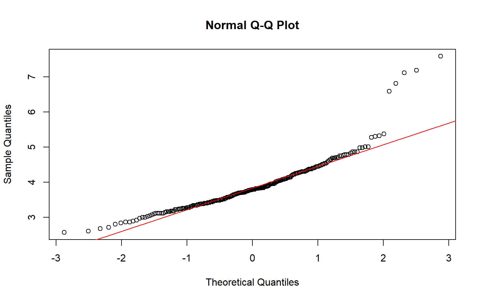


qqnorm(group1_transform)                  
qqline(group1_transform, col = "red")


shapiro_test_group2 <- shapiro.test(group2_transform)
shapiro_test_group2

    Shapiro-Wilk normality test

data:  group2_transform
W = 0.94436, p-value = 4.862e-08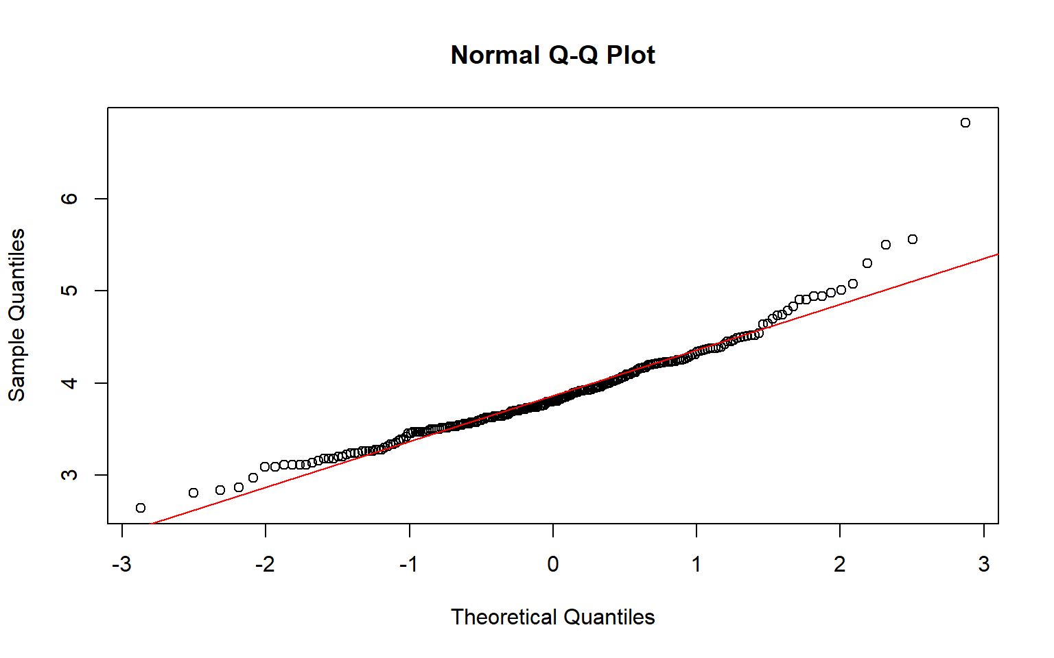


qqnorm(group2_transform)          
qqline(group2_transform, col = "red")


shapiro_test_group3 <- shapiro.test(group3_transform)
shapiro_test_group3

    Shapiro-Wilk normality test

data:  group3_transform
W = 0.88145, p-value < 2.2e-16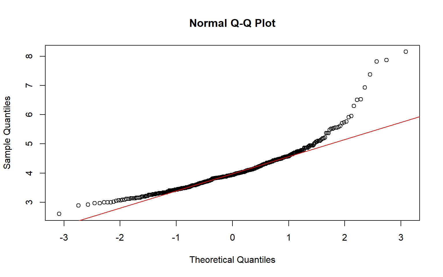


qqnorm(group3_transform)                  
qqline(group3_transform, col = "red")


# Levene test shoud be greater than 0.05 to indicate normal distribution
levene_test_result <- leveneTest(value ~ group, data = data_combined_chromatin)
levene_test_result
Levene's Test for Homogeneity of Variance (center = median)
       Df F value  Pr(>F)  
group   2  4.5851 0.01042 *
      983                  
---
Signif. codes:  0 '***' 0.001 '**' 0.01 '*' 0.05 '.' 0.1 ' ' 1


# Welch Anova test, doesn't assume equal variance or equal sample sizes
welch_anova_result <- oneway.test(value ~ group, data = data_combined_chromatin)
welch_anova_result

    One-way analysis of means (not assuming equal variances)

data:  value and group
F = 9.1355, num df = 2.00, denom df = 550.97, p-value = 0.000125


# Games-Howell test, doesn't assume equal variance or equal sample sizes
games_howell_result <- gamesHowellTest(value ~ group, data = data_combined_chromatin)
print(games_howell_result)
        Group 1 Group 2
Group 2 0.96622 -      
Group 3 0.00725 0.00024

Cytoplasm Significance


# Format the genes for the Chromatin Welch test

cytoplasm_genes <- filter(data_long_clean, Variable == "Cytoplasm") #Isolates the Chromatin Analysis

#---------------
# Chromatin | Separates based on Buffering score 

group1 <- filter(cytoplasm_genes, Buffering == "TB1") |>
  select(Value)
group2 <- filter(cytoplasm_genes, Buffering == "TB2") |>
  select(Value)
group3 <- filter(cytoplasm_genes, Buffering == "TB3") |>
  select(Value)

group1_transform <- log(as.numeric(unlist(group1)))
group2_transform <- log(as.numeric(unlist(group2)))
group3_transform <- log(as.numeric(unlist(group3)))


# Combine the groups into a data frame for testing
data_combined_cytoplasm <- data.frame(
  value = c(group1_transform, group2_transform, group3_transform),
  group = factor(rep(c("Group 1", "Group 2", "Group 3"), 
                     c(length(group1_transform), length(group2_transform), length(group3_transform))))
)

#--------------

# Check normality for each group with a Shapiro test and visualize with a qqline plot
shapiro_test_group1 <- shapiro.test(group1_transform)
shapiro_test_group1

    Shapiro-Wilk normality test

data:  group1_transform
W = 0.91866, p-value = 2.147e-10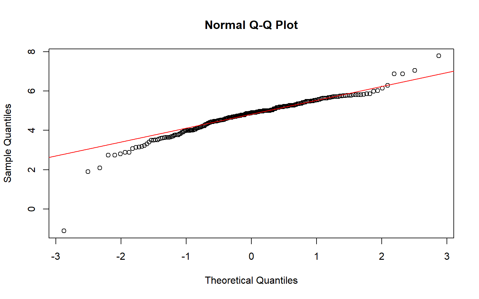


qqnorm(group1_transform)                  
qqline(group1_transform, col = "red")


shapiro_test_group2 <- shapiro.test(group2_transform)
shapiro_test_group2

    Shapiro-Wilk normality test

data:  group2_transform
W = 0.98306, p-value = 0.005115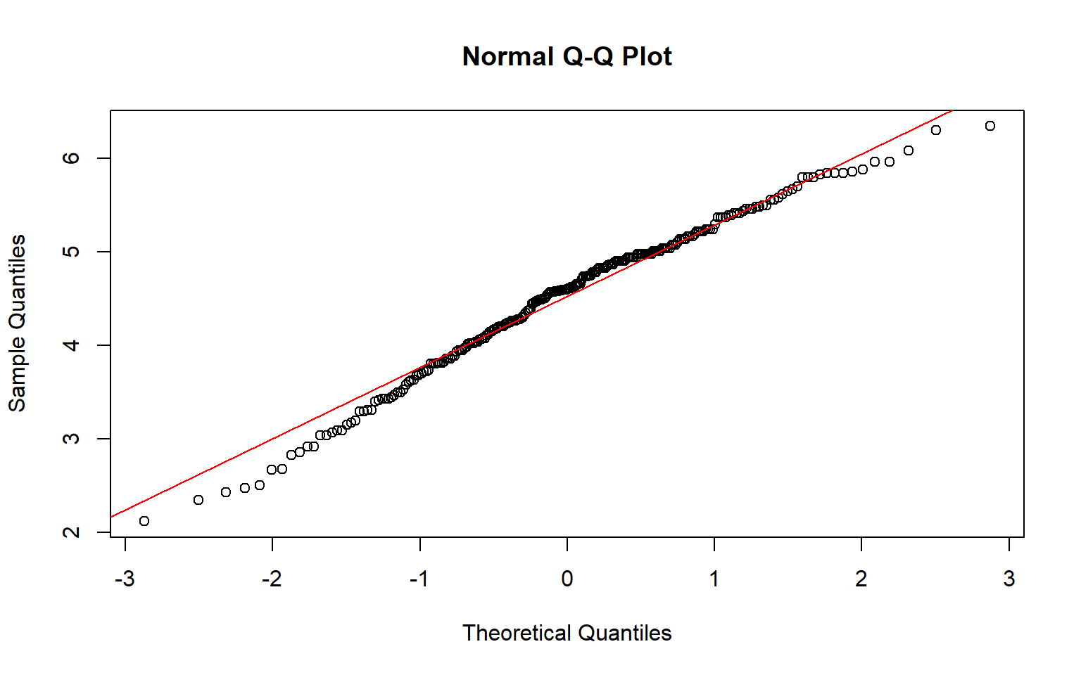


qqnorm(group2_transform)          
qqline(group2_transform, col = "red")


shapiro_test_group3 <- shapiro.test(group3_transform)
shapiro_test_group3

    Shapiro-Wilk normality test

data:  group3_transform
W = 0.95631, p-value = 6.551e-11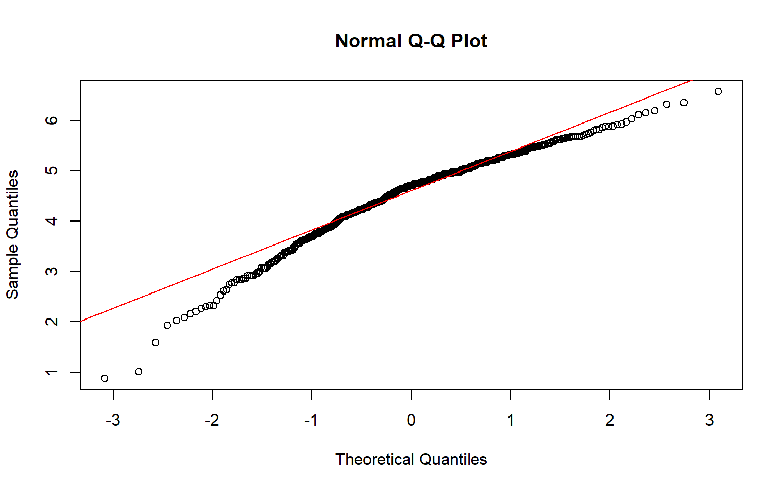


qqnorm(group3_transform)                  
qqline(group3_transform, col = "red")


# Levene test shoud be greater than 0.05 to indicate normal distribution
levene_test_result <- leveneTest(value ~ group, data = data_combined_cytoplasm)
levene_test_result
Levene's Test for Homogeneity of Variance (center = median)
       Df F value Pr(>F)
group   2  0.0639 0.9381
      983


# Welch Anova test, doesn't assume equal variance or equal sample sizes
welch_anova_result <- oneway.test(value ~ group, data = data_combined_cytoplasm)
welch_anova_result

    One-way analysis of means (not assuming equal variances)

data:  value and group
F = 6.5525, num df = 2.00, denom df = 525.62, p-value = 0.001546


# Games-Howell test, doesn't assume equal variance or equal sample sizes
games_howell_result <- gamesHowellTest(value ~ group, data = data_combined_cytoplasm)
print(games_howell_result)
        Group 1 Group 2
Group 2 0.0042  -      
Group 3 0.0029  0.9550

Nucleoplasm Significance


# Nucleoplasm Welch Anova Test

#---------------
# Format the genes for the Chromatin Welch test

nucleoplasm_genes <- filter(data_long_clean, Variable == "Nucleoplasm") #Isolates the Chromatin Analysis

#---------------
# Nucleoplasm | Separates based on Buffering score 

group1 <- filter(nucleoplasm_genes, Buffering == "TB1") |>
  select(Value)
group2 <- filter(nucleoplasm_genes, Buffering == "TB2") |>
  select(Value)
group3 <- filter(nucleoplasm_genes, Buffering == "TB3") |>
  select(Value)

group1_transform <- log(as.numeric(unlist(group1)))
group2_transform <- log(as.numeric(unlist(group2)))
group3_transform <- log(as.numeric(unlist(group3)))


# Combine the groups into a data frame for testing
data_combined_nucleoplasm <- data.frame(
  value = c(group1_transform, group2_transform, group3_transform),
  group = factor(rep(c("Group 1", "Group 2", "Group 3"), 
                     c(length(group1_transform), length(group2_transform), length(group3_transform))))
)

#--------------

# Check normality for each group with a Shapiro test and visualize with a qqline plot
shapiro_test_group1 <- shapiro.test(group1_transform)
shapiro_test_group1

    Shapiro-Wilk normality test

data:  group1_transform
W = 0.92656, p-value = 9.008e-10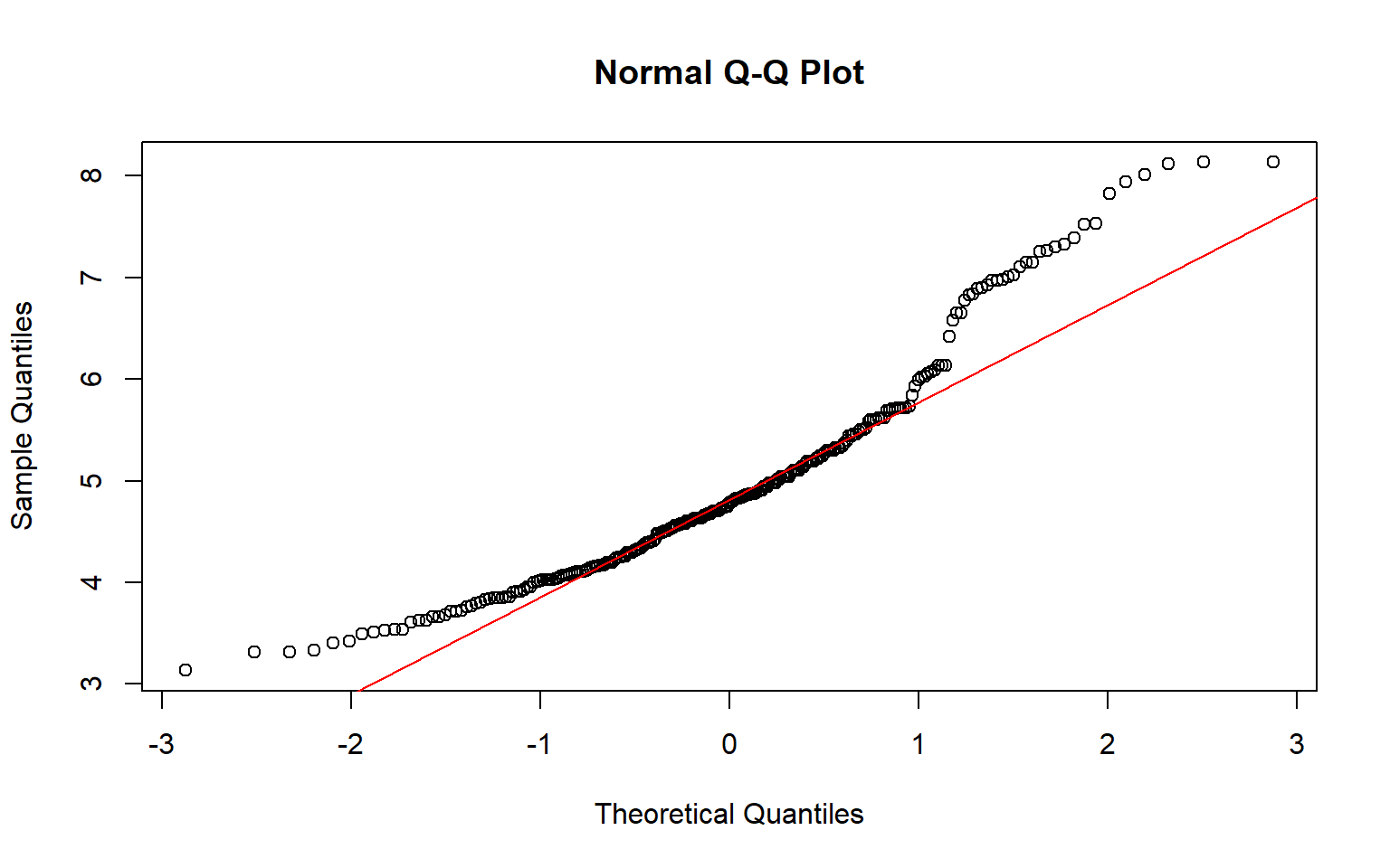


qqnorm(group1_transform)                  
qqline(group1_transform, col = "red")


shapiro_test_group2 <- shapiro.test(group2_transform)
shapiro_test_group2

    Shapiro-Wilk normality test

data:  group2_transform
W = 0.93833, p-value = 1.269e-08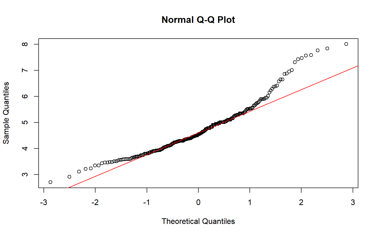


qqnorm(group2_transform)          
qqline(group2_transform, col = "red")


shapiro_test_group3 <- shapiro.test(group3_transform)
shapiro_test_group3

    Shapiro-Wilk normality test

data:  group3_transform
W = 0.9646, p-value = 1.602e-09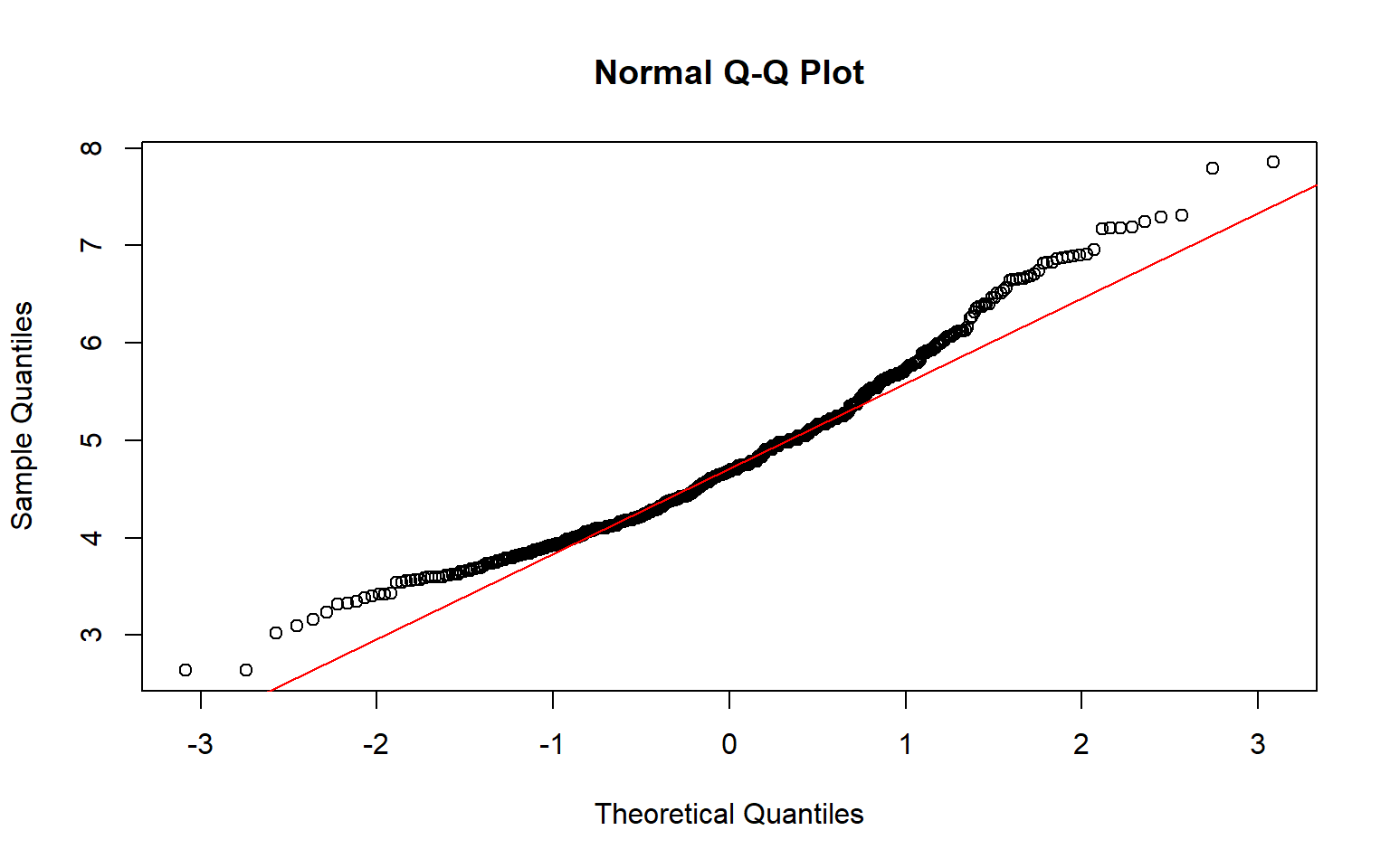


qqnorm(group3_transform)                  
qqline(group3_transform, col = "red")


# Levene test shoud be greater than 0.05 to indicate normal distribution
levene_test_result <- leveneTest(value ~ group, data = data_combined_nucleoplasm)
levene_test_result
Levene's Test for Homogeneity of Variance (center = median)
       Df F value Pr(>F)
group   2  1.6545 0.1917
      984


# Welch Anova test, doesn't assume equal variance or equal sample sizes
welch_anova_result <- oneway.test(value ~ group, data = data_combined_nucleoplasm)
welch_anova_result

    One-way analysis of means (not assuming equal variances)

data:  value and group
F = 3.9033, num df = 2.00, denom df = 502.58, p-value = 0.02079


# Games-Howell test, doesn't assume equal variance or equal sample sizes
games_howell_result <- gamesHowellTest(value ~ group, data = data_combined_nucleoplasm)
print(games_howell_result)
        Group 1 Group 2
Group 2 0.016   -      
Group 3 0.093   0.467

Polysome Significance


# Untranslated Cytoplasm Welch Anova Test

#---------------
# Format the genes for the Chromatin Welch test

untranslated_cytoplasm_genes <- filter(data_long_clean, Variable == "Untranslated Cytoplasm") #Isolates the Chromatin Analysis

#---------------
# Untranslated Cytoplasm | Separates based on Buffering score 

group1 <- filter(untranslated_cytoplasm_genes, Buffering == "TB1") |>
  select(Value)
group2 <- filter(untranslated_cytoplasm_genes, Buffering == "TB2") |>
  select(Value)
group3 <- filter(untranslated_cytoplasm_genes, Buffering == "TB3") |>
  select(Value)

group1_transform <- log(as.numeric(unlist(group1)))
group2_transform <- log(as.numeric(unlist(group2)))
group3_transform <- log(as.numeric(unlist(group3)))


# Combine the groups into a data frame for testing
data_combined_untranslated_cytoplasm <- data.frame(
  value = c(group1_transform, group2_transform, group3_transform),
  group = factor(rep(c("Group 1", "Group 2", "Group 3"), 
                     c(length(group1_transform), length(group2_transform), length(group3_transform))))
)

#--------------

# Check normality for each group with a Shapiro test and visualize with a qqline plot
shapiro_test_group1 <- shapiro.test(group1_transform)
shapiro_test_group1

    Shapiro-Wilk normality test

data:  group1_transform
W = 0.96518, p-value = 9.786e-06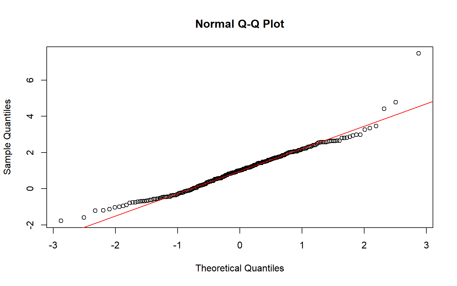


qqnorm(group1_transform)                  
qqline(group1_transform, col = "red")


shapiro_test_group2 <- shapiro.test(group2_transform)
shapiro_test_group2

    Shapiro-Wilk normality test

data:  group2_transform
W = 0.90564, p-value = 2.702e-11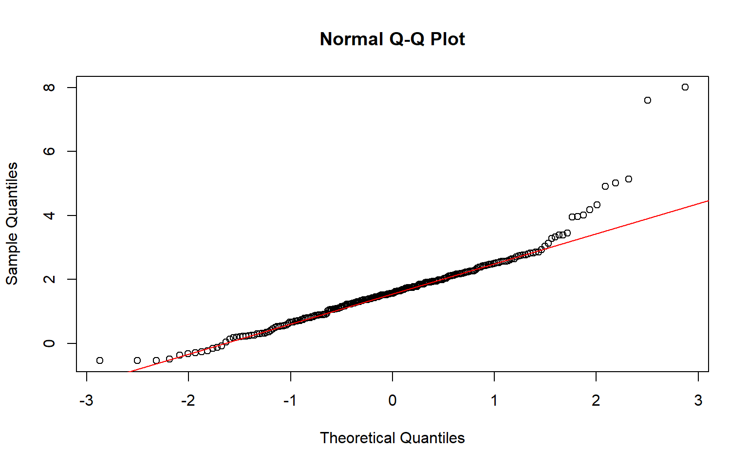


qqnorm(group2_transform)          
qqline(group2_transform, col = "red")


shapiro_test_group3 <- shapiro.test(group3_transform)
shapiro_test_group3

    Shapiro-Wilk normality test

data:  group3_transform
W = 0.92653, p-value = 8.967e-15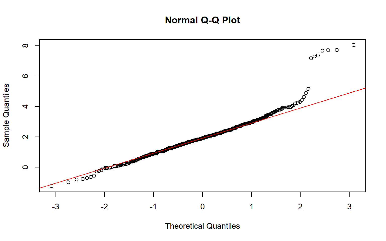


qqnorm(group3_transform)                  
qqline(group3_transform, col = "red")


# Levene test shoud be greater than 0.05 to indicate normal distribution
levene_test_result <- leveneTest(value ~ group, data = data_combined_untranslated_cytoplasm)
levene_test_result
Levene's Test for Homogeneity of Variance (center = median)
       Df F value Pr(>F)
group   2  2.0532 0.1289
      981


# Welch Anova test, doesn't assume equal variance or equal sample sizes
welch_anova_result <- oneway.test(value ~ group, data = data_combined_untranslated_cytoplasm)
welch_anova_result

    One-way analysis of means (not assuming equal variances)

data:  value and group
F = 51.848, num df = 2.00, denom df = 534.41, p-value < 2.2e-16


# Games-Howell test, doesn't assume equal variance or equal sample sizes
games_howell_result <- gamesHowellTest(value ~ group, data = data_combined_untranslated_cytoplasm)
print(games_howell_result)
        Group 1 Group 2
Group 2 1.3e-08 -      
Group 3 1.6e-10 0.00087

Brief Summary

According to the results of the Games-Howell test, the RNA of buffered genes spend significantly more time in the chromatin, polysome, and possibly the cytoplasm than non-buffered genes